The function and the study of its features occupies one of the key chapters in modern mathematics. The main component of any function is graphs depicting not only its properties, but also the parameters of the derivative of this function. Let's understand this difficult topic. So what is the best way to find the maximum and minimum points of a function?
Function: definition
Any variable that in some way depends on the values of another quantity can be called a function. For example, the function f(x 2) is quadratic and determines the values for the entire set x. Let's say that x = 9, then the value of our function will be equal to 9 2 = 81.
Functions come in many different types: logical, vector, logarithmic, trigonometric, numeric and others. They were studied by such outstanding minds as Lacroix, Lagrange, Leibniz and Bernoulli. Their works serve as a mainstay in modern ways of studying functions. Before finding the minimum points, it is very important to understand the very meaning of the function and its derivative.
Derivative and its role
All functions depend on their variables, which means that they can change their value at any time. On the graph, this will be depicted as a curve that either falls or rises along the ordinate axis (this is the whole set of “y” numbers along the vertical graph). So, determining the maximum and minimum points of a function is precisely related to these “oscillations”. Let us explain what this relationship is.

The derivative of any function is graphed in order to study its basic characteristics and calculate how quickly the function changes (i.e. changes its value depending on the variable "x"). At the moment when the function increases, the graph of its derivative will also increase, but at any second the function can begin to decrease, and then the graph of the derivative will decrease. Those points at which the derivative changes from a minus sign to a plus sign are called minimum points. In order to know how to find minimum points, you should better understand
How to calculate derivative?
The definition and functions imply several concepts from In general, the very definition of a derivative can be expressed as follows: this is the quantity that shows the rate of change of the function.

The mathematical way of determining it seems complicated for many students, but in reality everything is much simpler. You just need to follow the standard plan for finding the derivative of any function. Below we describe how you can find the minimum point of a function without applying the rules of differentiation and without memorizing the table of derivatives.
- You can calculate the derivative of a function using a graph. To do this, you need to depict the function itself, then take one point on it (point A in the figure). Draw a line vertically down to the abscissa axis (point x 0), and at point A draw a tangent to the graph of the function. The x-axis and the tangent form a certain angle a. To calculate the value of how quickly a function increases, you need to calculate the tangent of this angle a.
- It turns out that the tangent of the angle between the tangent and the direction of the x-axis is the derivative of the function in a small area with point A. This method is considered a geometric method for determining the derivative.

Methods for studying function
In the school mathematics curriculum, it is possible to find the minimum point of a function in two ways. We have already discussed the first method using a graph, but how can we determine the numerical value of the derivative? To do this, you will need to learn several formulas that describe the properties of the derivative and help convert variables like “x” into numbers. The following method is universal, so it can be applied to almost all types of functions (both geometric and logarithmic).
- It is necessary to equate the function to the derivative function, and then simplify the expression using the rules of differentiation.
- In some cases, when given a function in which the variable “x” is in the divisor, it is necessary to determine the range of acceptable values, excluding the point “0” from it (for the simple reason that in mathematics one should never divide by zero).
- After this, you should transform the original form of the function into a simple equation, equating the entire expression to zero. For example, if the function looked like this: f(x) = 2x 3 +38x, then according to the rules of differentiation its derivative is equal to f"(x) = 3x 2 +1. Then we transform this expression into an equation of the following form: 3x 2 +1 = 0 .
- After solving the equation and finding the “x” points, you should plot them on the x-axis and determine whether the derivative in these sections between the marked points is positive or negative. After the designation, it will become clear at what point the function begins to decrease, that is, changes sign from minus to the opposite. It is in this way that you can find both the minimum and maximum points.
Rules of differentiation
The most basic component in studying a function and its derivative is knowledge of the rules of differentiation. Only with their help can you transform cumbersome expressions and large complex functions. Let's get acquainted with them, there are quite a lot of them, but they are all very simple due to the natural properties of both power and logarithmic functions.
- The derivative of any constant is equal to zero (f(x) = 0). That is, the derivative f(x) = x 5 + x - 160 will take the following form: f" (x) = 5x 4 +1.
- Derivative of the sum of two terms: (f+w)" = f"w + fw".
- Derivative of a logarithmic function: (log a d)" = d/ln a*d. This formula applies to all types of logarithms.
- Derivative of the power: (x n)"= n*x n-1. For example, (9x 2)" = 9*2x = 18x.
- The derivative of the sinusoidal function: (sin a)" = cos a. If the sin of angle a is 0.5, then its derivative is √3/2.
Extremum points
We have already discussed how to find minimum points, but there is also the concept of maximum points of a function. If the minimum denotes those points at which the function changes from a minus sign to a plus, then the maximum points are those points on the x-axis at which the derivative of the function changes from plus to the opposite - minus.

You can find it using the method described above, but you should take into account that they indicate those areas in which the function begins to decrease, that is, the derivative will be less than zero.
In mathematics, it is customary to generalize both concepts, replacing them with the phrase “points of extrema.” When a task asks you to determine these points, it means that you need to calculate the derivative of a given function and find the minimum and maximum points.
Theorem. (a necessary condition for the existence of an extremum) If the function f(x) is differentiable at the point x = x 1 and the point x 1 is an extremum point, then the derivative of the function vanishes at this point.
Proof. Let us assume that the function f(x) has a maximum at the point x = x 1.
Then for sufficiently small positive Dх>0 the following inequality is true:
A-priory:
![]()
Those. if Dх®0, but Dх<0, то f¢(x 1) ³ 0, а если Dх®0, но Dх>0, then f¢(x 1) £ 0.
And this is possible only if at Dх®0 f¢(x 1) = 0.
For the case if the function f(x) has a minimum at point x 2, the theorem is proved in a similar way.
The theorem has been proven.
Consequence. The reverse statement is not true. If the derivative of a function at a certain point is equal to zero, this does not mean that the function has an extremum at this point. An eloquent example of this is the function y = x 3, the derivative of which at the point x = 0 is equal to zero, but at this point the function only has an inflection, and not a maximum or minimum.
Definition. Critical points functions are the points at which the derivative of the function does not exist or is equal to zero.
The theorem discussed above gives us the necessary conditions for the existence of an extremum, but this is not enough.
Example: f(x) = ôxô Example: f(x) =
 y y
y y
At the point x = 0 the function has a minimum, but at the point x = 0 the function has neither
has no derivative. maximum, no minimum, no production
Generally speaking, the function f(x) may have an extremum at points where the derivative does not exist or is equal to zero.
Theorem. (Sufficient conditions for the existence of an extremum)
Let the function f(x) be continuous in the interval (a, b), which contains the critical point x 1, and differentiable at all points of this interval (except, perhaps, the point x 1 itself).
If, when passing through the point x 1 from left to right, the derivative of the function f¢(x) changes sign from “+” to “-“, then at the point x = x 1 the function f(x) has a maximum, and if the derivative changes sign from “- “ to “+” - then the function has a minimum.
Proof.
Let 
According to Lagrange's theorem: f(x) – f(x 1) = f¢(e)(x – x 1), where x< e < x 1 .
Then: 1) If x< x 1 , то e < x 1 ; f¢(e)>0; f¢(e)(x – x 1)<0, следовательно
f(x) – f(x 1)<0 или f(x) < f(x 1).
2) If x > x 1, then e > x 1 f¢(e)<0; f¢(e)(x – x 1)<0, следовательно
f(x) – f(x 1)<0 или f(x) < f(x 1).
Since the answers coincide, we can say that f(x)< f(x 1) в любых точках вблизи х 1 , т.е. х 1 – точка максимума.
The proof of the theorem for the minimum point is similar.
The theorem has been proven.
Based on the above, you can develop a unified procedure for finding the largest and smallest values of a function on a segment:
1) Find the critical points of the function.
2) Find the values of the function at critical points.
3) Find the values of the function at the ends of the segment.
4) Select the largest and smallest among the obtained values.
Studying a function for an extremum using
derivatives of higher orders.
Let at the point x = x 1 f¢(x 1) = 0 and f¢¢(x 1) exists and is continuous in some neighborhood of the point x 1.
Theorem. If f¢(x 1) = 0, then the function f(x) at the point x = x 1 has a maximum if f¢¢(x 1)<0 и минимум, если f¢¢(x 1)>0.
Proof.
Let f¢(x 1) = 0 and f¢¢(x 1)<0. Т.к. функция f(x) непрерывна, то f¢¢(x 1) будет отрицательной и в некоторой малой окрестности точки х 1 .
Because f¢¢(x) = (f¢(x))¢< 0, то f¢(x) убывает на отрезке, содержащем точку х 1 , но f¢(x 1)=0, т.е. f¢(x) >0 at x
For the case of a minimum function, the theorem is proved in a similar way.
If f¢¢(x) = 0, then the nature of the critical point is unknown. Further research is required to determine it.
Convexity and concavity of a curve.
Inflection points.
Definition. The curve is convex up on the interval (a, b) if all its points lie below any of its tangents on this interval. A curve convex upward is called convex, and a curve facing convexly downward is called concave.
 at
at
The figure shows an illustration of the above definition.
Theorem 1. If at all points of the interval (a, b) the second derivative of the function f(x) is negative, then the curve y = f(x) is convex upward (convex).
Proof. Let x 0 О (a, b). Let's draw a tangent to the curve at this point.
Curve equation: y = f(x);
Tangent equation:
It must be proven that .
By Lagrange’s theorem for f(x) – f(x 0): , x 0< c < x.
According to Lagrange's theorem for ![]()
Let x > x 0 then x 0< c 1 < c < x. Т.к. x – x 0 >0 and c – x 0 > 0, and in addition, by condition
Hence, .
Let x< x 0 тогда x < c < c 1 < x 0 и x – x 0 < 0, c – x 0 < 0, т.к. по условию то
It is similarly proven that if f¢¢(x) > 0 on the interval (a, b), then the curve y=f(x) is concave on the interval (a, b).
The theorem has been proven.
Definition. The point separating the convex part of the curve from the concave part is called inflection point.
Obviously, at the inflection point the tangent intersects the curve.
Theorem 2. Let the curve be defined by the equation y = f(x). If the second derivative f¢¢(a) = 0 or f¢¢(a) does not exist and when passing through the point x = a f¢¢(x) changes sign, then the point of the curve with the abscissa x = a is an inflection point.
Proof. 1) Let f¢¢(x)< 0 при х < a и f¢¢(x) >0 for x > a. Then at
x< a кривая выпукла, а при x >a the curve is concave, i.e. point x = a – inflection point.
2) Let f¢¢(x) > 0 for x< b и f¢¢(x) < 0 при x < b. Тогда при x < b кривая обращена выпуклостью вниз, а при x >b – convex upward. Then x = b is the inflection point.
The theorem has been proven.
Asymptotes.
When studying functions, it often happens that when the x-coordinate of a point on a curve moves to infinity, the curve indefinitely approaches a certain straight line.
Definition. The straight line is called asymptote curve if the distance from the variable point of the curve to this straight line tends to zero as the point moves to infinity.
It should be noted that not every curve has an asymptote. Asymptotes can be straight or oblique. Studying functions for the presence of asymptotes is of great importance and allows you to more accurately determine the nature of the function and the behavior of the curve graph.
Generally speaking, a curve, indefinitely approaching its asymptote, can intersect it, and not at one point, as shown in the graph of the function below ![]() . Its oblique asymptote is y = x.
. Its oblique asymptote is y = x.

Let us consider in more detail the methods for finding the asymptotes of curves.
Vertical asymptotes.
From the definition of an asymptote it follows that if or or , then the straight line x = a is the asymptote of the curve y = f(x).
For example, for a function, the line x = 5 is a vertical asymptote.
Oblique asymptotes.
Suppose that the curve y = f(x) has a slanted asymptote y = kx + b.

 |
Let us denote the point of intersection of the curve and the perpendicular to the asymptote - M, P - the point of intersection of this perpendicular with the asymptote. Let us denote the angle between the asymptote and the Ox axis as j. The perpendicular MQ to the Ox axis intersects the asymptote at point N.
Then MQ = y is the ordinate of the point on the curve, NQ = is the ordinate of point N on the asymptote.
According to the condition: , ÐNMP = j, .
Angle j is constant and not equal to 90 0, then
Then ![]() .
.
So, the straight line y = kx + b is the asymptote of the curve. To accurately determine this line, it is necessary to find a way to calculate the coefficients k and b.
In the resulting expression we take x out of brackets:
![]()
Because x®¥, then ![]() , because b = const, then
, because b = const, then ![]() .
.
Then ![]() , hence,
, hence,
 .
.
Because ![]() , That
, That ![]() , hence,
, hence,

![]()
Note that horizontal asymptotes are a special case of oblique asymptotes for k = 0.
Example. ![]() .
.
1) Vertical asymptotes: y®+¥ x®0-0: y®-¥ x®0+0, therefore, x = 0 is a vertical asymptote.
2) Oblique asymptotes:
![]()
Thus, the straight line y = x + 2 is an oblique asymptote.
Let's plot the function:

Example. Find asymptotes and graph the function.
The lines x = 3 and x = -3 are vertical asymptotes of the curve.
Let's find the oblique asymptotes: ![]()

y = 0 – horizontal asymptote.

Example. Find asymptotes and graph the function ![]() .
.
The straight line x = -2 is the vertical asymptote of the curve.
Let's find the oblique asymptotes.

In total, the straight line y = x – 4 is an oblique asymptote.

Function study scheme
The function research process consists of several stages. For the most complete understanding of the behavior of the function and the nature of its graph, it is necessary to find:
1) The domain of existence of the function.
This concept includes both the domain of values and the domain of definition of a function.
2) Breaking points. (If available).
3) Intervals of increase and decrease.
4) Maximum and minimum points.
5) The maximum and minimum value of a function on its domain of definition.
6) Areas of convexity and concavity.
7) Inflection points (if any).
8) Asymptotes (if any).
9) Building a graph.
Let's look at the application of this scheme using an example.
Example. Explore the function and build its graph.
We find the domain of existence of the function. It's obvious that domain of definition function is the area (-¥; -1) È (-1; 1) È (1; ¥).
In turn, it is clear that the straight lines x = 1, x = -1 are vertical asymptotes crooked.
Range of values of this function is the interval (-¥; ¥).
Break points functions are points x = 1, x = -1.
We find critical points.
Let's find the derivative of the function
Critical points: x = 0; x = - ; x = ; x = -1; x = 1.
Let's find the second derivative of the function
Let us determine the convexity and concavity of the curve at intervals.
-¥ < x < - , y¢¢ < 0, кривая выпуклая
- < x < -1, y¢¢ < 0, кривая выпуклая
1 < x < 0, y¢¢ >0, concave curve
0 < x < 1, y¢¢ < 0, кривая выпуклая
1 < x < , y¢¢ >0, concave curve
< x < ¥, y¢¢ >0, concave curve
Finding the gaps increasing And descending functions. To do this, we determine the signs of the derivative of the function on intervals.
-¥ < x < - , y¢ >0, function is increasing
- < x < -1, y¢ < 0, функция убывает
1 < x < 0, y¢ < 0, функция убывает
0 < x < 1, y¢ < 0, функция убывает
1 < x < , y¢ < 0, функция убывает
< x < ¥, y¢¢ >0, function is increasing
It can be seen that the point x = - is a point maximum, and point x = is a point minimum. The function values at these points are equal to -3 /2 and 3 /2, respectively.
About vertical asymptotes has already been said above. Now let's find oblique asymptotes.


In total, the equation of the oblique asymptote is y = x.
Let's build schedule Features:

Functions of several variables
When considering functions of several variables, we will limit ourselves to a detailed description of the functions of two variables, since all the results obtained will be valid for functions of an arbitrary number of variables.
Definition: If each pair of mutually independent numbers (x, y) from a certain set, according to some rule, is associated with one or more values of the variable z, then the variable z is called a function of two variables.
Definition: If a pair of numbers (x, y) corresponds to one value z, then the function is called unambiguous, and if more than one, then – polysemantic.
Definition: Domain of definition function z is the set of pairs (x, y) for which function z exists.
Definition: Neighborhood of a point M 0 (x 0, y 0) of radius r is the set of all points (x, y) that satisfy the condition ![]() .
.
Definition: The number A is called limit function f(x, y) as the point M(x, y) tends to the point M 0 (x 0, y 0), if for each number e > 0 there is a number r > 0 such that for any point M(x, y), for which the condition is true
the condition is also true ![]() .
.
Write down: ![]()
Definition: Let the point M 0 (x 0, y 0) belong to the domain of definition of the function f(x, y). Then the function z = f(x, y) is called continuous at point M 0 (x 0, y 0), if
![]() (1)
(1)
and the point M(x, y) tends to the point M 0 (x 0, y 0) in an arbitrary manner.
If at any point condition (1) is not satisfied, then this point is called break point functions f(x, y). This may be in the following cases:
1) The function z = f(x, y) is not defined at the point M 0 (x 0, y 0).
2) There is no limit.
3) This limit exists, but it is not equal to f(x 0 , y 0).
Property. If the function f(x, y, …) is defined and continuous in a closed and
bounded domain D, then in this domain there is at least one point
N(x 0 , y 0 , …), such that for the remaining points the inequality is true
f(x 0 , y 0 , …) ³ f(x, y, …)
as well as point N 1 (x 01, y 01, ...), such that for all other points the inequality is true
f(x 01 , y 01 , …) £ f(x, y, …)
then f(x 0 , y 0 , …) = M – highest value functions, and f(x 01 , y 01 , ...) = m – smallest value functions f(x, y, …) in domain D.
A continuous function in a closed and bounded domain D reaches its largest value at least once and its smallest value once.
Property. If the function f(x, y, …) is defined and continuous in a closed bounded domain D, and M and m are, respectively, the largest and smallest values of the function in this domain, then for any point m О there is a point
N 0 (x 0 , y 0 , …) such that f(x 0 , y 0 , …) = m.
Simply put, a continuous function takes in the domain D all intermediate values between M and m. A consequence of this property can be the conclusion that if the numbers M and m are of different signs, then in the domain D the function vanishes at least once.
Property.
Function f(x, y, …), continuous in a closed bounded domain D, limited in this region, if there is a number K such that for all points in the region the inequality is true ![]() .
.
Property. If a function f(x, y, …) is defined and continuous in a closed bounded domain D, then it uniformly continuous in this area, i.e. for any positive number e there is a number D > 0 such that for any two points (x 1, y 1) and (x 2, y 2) of the region located at a distance less than D, the inequality holds
The above properties are similar to the properties of functions of one variable that are continuous on an interval. See Properties of functions continuous on an interval.
Derivatives and differentials of functions
several variables.
Definition. Let the function z = f(x, y) be given in some domain. Let's take an arbitrary point M(x, y) and set the increment Dx to the variable x. Then the quantity D x z = f(x + Dx, y) – f(x, y) is called partial increment of the function in x.
You can write down
![]() .
.
Then it's called partial derivative functions z = f(x, y) in x.
Designation: ![]()
The partial derivative of a function with respect to y is determined similarly.
![]()
Geometric sense the partial derivative (let's say) is the tangent of the angle of inclination of the tangent drawn at point N 0 (x 0, y 0, z 0) to the section of the surface by the plane y = y 0.
Full increment and full differential.
tangent plane
Let N and N 0 be points of this surface. Let's draw a straight line NN 0. The plane that passes through the point N 0 is called tangent plane to the surface if the angle between the secant NN 0 and this plane tends to zero, when the distance NN 0 tends to zero.
Definition. Normal to the surface at point N 0 is a straight line passing through point N 0 perpendicular to the tangent plane to this surface.
At any point the surface has either only one tangent plane or does not have it at all.
If the surface is given by the equation z = f(x, y), where f(x, y) is a function differentiable at the point M 0 (x 0, y 0), the tangent plane at the point N 0 (x 0,y 0, ( x 0 ,y 0)) exists and has the equation:
The equation of the normal to the surface at this point is:
![]()
Geometric sense the total differential of a function of two variables f(x, y) at the point (x 0, y 0) is the increment of the applicate (z coordinates) of the tangent plane to the surface when moving from the point (x 0, y 0) to the point (x 0 + Dx, y 0 +Dу).
As you can see, the geometric meaning of the total differential of a function of two variables is a spatial analogue of the geometric meaning of the differential of a function of one variable.
Example. Find the equations of the tangent plane and normal to the surface
at point M(1, 1, 1).
![]()
![]()
Tangent plane equation:
Normal equation:
![]()
Approximate calculations using total differentials.
The total differential of the function u is equal to:
![]()
The exact value of this expression is 1.049275225687319176.
Partial derivatives of higher orders.
If a function f(x, y) is defined in some domain D, then its partial derivatives will also be defined in the same domain or part of it.
We will call these derivatives first order partial derivatives.
The derivatives of these functions will be second order partial derivatives.
![]()
![]()
Continuing to differentiate the resulting equalities, we obtain partial derivatives of higher orders.
1°. Determination of the extremum of a function.
The concepts of maximum, minimum, and extremum of a function of two variables are similar to the corresponding concepts of a function of one independent variable.
Let the function z =f (x ; y) defined in some area D dot N (x 0 ;y 0) D.
Dot (x 0 ;y 0) called a point maximum functions z= f (x ;y ), if there is such an -neighborhood of the point (x 0 ;y 0), that for each point (x;y), different from (x 0 ;y 0) from this neighborhood the inequality holds f (x ;y)< f (x 0 ;y 0). In Figure 12: N 1 - maximum point, a N 2 - minimum point of the function z =f (x ;y).
The point is determined similarly minimum functions: for all points (x 0 ;y 0), different from (x 0 ;y 0), from d -neighborhood of a point (x 0 ;y 0) inequality holds: f (x 0 ;y 0) >f (x 0 ;y 0).
The extremum of a function of three or more variables is determined similarly.
The value of the function at the maximum (minimum) point is called maximum (minimum) functions.
The maximum and minimum of a function is called extremes.
Note that, by definition, the extremum point of the function lies inside the domain of definition of the function; maximum and minimum have local(local) character: the value of a function at a point (x 0 ;y 0) is compared with its values at points sufficiently close to (x 0 ;y 0). In area D a function may have several extrema or none.
2°. Necessary conditions for an extremum.
Let us consider the conditions for the existence of an extremum of a function.
Geometrically equalities f"y (x 0 ;y 0)= 0 and f"y (x 0 ;y 0) = 0 means that at the extremum point of the function z = f (x ; y) tangent plane to the surface representing the function f (x ; y), parallel to the plane Oh hoo since the equation of the tangent plane is z =z 0.
Comment. A function can have an extremum at points where at least one of the partial derivatives does not exist. For example, the function ![]() has a maximum at the point ABOUT(0;0), but has no partial derivatives at this point.
has a maximum at the point ABOUT(0;0), but has no partial derivatives at this point.
The point at which the first order partial derivatives of the function z = f (x ;y) are equal to zero, i.e. f"x = 0, f" y = 0, called stationary point functions z.
Stationary points and points at which at least one partial derivative does not exist are called critical points.
At critical points, the function may or may not have an extremum. The equality of partial derivatives to zero is a necessary but not sufficient condition for the existence of an extremum. Consider, for example, the function z = hu. For it, the point 0(0; 0) is critical (it turns to zero). However, the extremum function in it is z = xy does not have, because in a sufficiently small neighborhood of the point O(0;0) there are points for which z> 0 (points of the 1st and 3rd quarters) and z< 0 (points of the II and IV quarters).
Thus, to find the extrema of a function in a given area, it is necessary to subject each critical point of the function to additional research.
Stationary points are found by solving the system of equations
|
fx (x, y) = 0, f"y (x, y) = 0 |
(necessary conditions for an extremum).
System (1) is equivalent to one equation df(x, y)=0. In general, at the extremum point P(a, b) functions f(x, y) or df(x, y)=0, or df(a, b) does not exist.
3°. Sufficient conditions for an extremum. Let P(a;b)- stationary point of the function f(x,y), i.e. . df(a, b) = 0. Then:
and if d2f (a, b)< 0 at , then f(a, b) There is maximum functions f (x, y);
b) if d2f (a, b) > 0 at , then f(a, b)There is minimum functions f (x,y);
c) if d2f (a, b) changes sign, then f (a, b) is not an extremum of the function f (x, y).
The given conditions are equivalent to the following: let ![]() And . Let's compose discriminant
Δ=AC -B².
And . Let's compose discriminant
Δ=AC -B².
1) if Δ > 0, then the function has an extremum at the point P(a;b) namely, the maximum if A<0 (or WITH<0 ), and a minimum if A>0(or С>0);
2) if Δ< 0, то экстремума в точке P(a;b) No;
3) if Δ =0, then the question of the presence of an extremum of the function at the point P(a;b) remains open (further research required).
4°. The case of a function of several variables. For a function of three or more variables, the necessary conditions for the existence of an extremum are similar to conditions (1), and the sufficient conditions are similar to conditions a), b), c) 3°.
Example. Examine the extremum function z=x³+3xy²-15x-12y.
Solution. Let's find partial derivatives and create a system of equations (1):
![]()
Solving the system, we obtain four stationary points:
Let's find the 2nd order derivatives
and create a discriminant Δ=AC - B² for each stationary point.
1) For point:  , Δ=AC-B²=36-144<0
. This means there is no extremum at the point.
, Δ=AC-B²=36-144<0
. This means there is no extremum at the point.
2) For point P2: A=12, B=6, C=12; Δ=144-36>0, A>0. At point P2 the function has a minimum. This minimum is equal to the value of the function at x=2, y=1: zmin=8+6-30-12=-28.
3) For point: A= -6, B=-12, C= -6; Δ = 36-144<0 . There is no extreme.
4) For point P 4: A=-12, B=-6, C=-12; Δ=144-36>0. At point P4 the function has a maximum equal to Zmax=-8-6+30+12=28.
5°. Conditional extremum. In the simplest case conditional extremum functions f(x,y) is the maximum or minimum of this function, achieved under the condition that its arguments are related by the equation φ(x,y)=0 (connection equation). To find the conditional extremum of a function f(x, y) in the presence of a relation φ(x,y) = 0, constitute the so-called Lagrange function
F (x,y )=f (x,y )+λφ (x,y ),
where λ is an undefined constant factor, and the usual extremum of this auxiliary function is sought. The necessary conditions for an extremum are reduced to a system of three equations
|
|

with three unknowns x, y, λ, from which these unknowns can, generally speaking, be determined.
The question of the existence and nature of the conditional extremum is resolved based on studying the sign of the second differential of the Lagrange function
for the value system under test x, y, λ, obtained from (2) provided that dx And dу related by the equation
![]() .
.
Namely, the function f(x,y) has a conditional maximum if d²F< 0, and a conditional minimum if d²F>0. In particular, if the discriminant Δ for the function F(x,y) is positive at a stationary point, then at this point there is a conditional maximum of the function f(x, y), If A< 0 (or WITH< 0), and a conditional minimum if A > O(or С>0).
Similarly, the conditional extremum of a function of three or more variables is found in the presence of one or more connection equations (the number of which, however, must be less than the number of variables). Here we have to introduce as many uncertain factors into the Lagrange function as there are coupling equations.
Example. Find the extremum of the function z =6-4x -3y provided that the variables X And at satisfy the equation x²+y²=1.
Solution. Geometrically, the problem comes down to finding the largest and smallest values of the applicate z plane z=6 - 4x - Zu for the points of intersection of it with the cylinder x2+y2=1.
Compiling the Lagrange function F(x,y)=6 -4x -3y+λ(x2+y2 -1).
We have ![]() . The necessary conditions give the system of equations
. The necessary conditions give the system of equations
solving which we find:
![]()
![]() .
.
![]() ,
,
d²F =2λ (dx²+dy²).
If and , then d²F >0, and, therefore, at this point the function has a conditional minimum. If ![]() and , then d²F<0,
and, therefore, at this point the function has a conditional maximum.
and , then d²F<0,
and, therefore, at this point the function has a conditional maximum.
Thus,

6°. The largest and smallest values of a function.
Let the function z =f (x ; y) defined and continuous in a limited closed region . Then she reaches at some points your greatest M and the least T values (so-called global extremum). These values are achieved by the function at points located inside the region , or at points lying on the boundary of the region.
Consider the function y = f(x), which is considered on the interval (a, b).
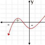
If it is possible to indicate a b-neighborhood of a point x1 belonging to the interval (a, b) such that for all x (x1, b), the inequality f(x1) > f(x) holds, then y1 = f1(x1) is called maximum of the function y = f(x) see fig.
We denote the maximum of the function y = f(x) by max f(x). If it is possible to indicate a b-neighborhood of a point x2 belonging to the interval (a, b) such that for all x it belongs to O (x2, 6), x is not equal to x2, the inequality holds f(x2)< f(x) , then y2= f(x2) is called the minimum of the function y-f(x) (see figure).
For an example of finding the maximum, see the following video
Minimum functions
We denote the minimum of the function y = f(x) by min f(x). In other words, maximum or minimum of a function y = f(x) called its value that is greater (less) than all other values accepted at points sufficiently close to the given one and different from it.
Note 1. Maximum function, defined by the inequality is called a strict maximum; the non-strict maximum is determined by the inequality f(x1) > = f(x2)
Note 2. have a local character (these are the largest and smallest values of the function in a sufficiently small neighborhood of the corresponding point); individual minima of a function may be greater than the maxima of the same function
 As a result, the maximum (minimum) of the function is called local maximum(local minimum) in contrast to the absolute maximum (minimum) - the largest (smallest) value in the domain of definition of the function.
The maximum and minimum of a function are called extremum . Extrema in are found to construct graphs of functions
Latin extremum means "extreme" meaning. The value of the argument x at which the extremum is reached is called the extremum point. The necessary condition for an extremum is expressed by the following theorem.
Theorem. At the extremum point of the differentiable function, its derivative is equal to zero.
The theorem has a simple geometric meaning: the tangent to the graph of the differentiable function at the corresponding point is parallel to the Ox axis
meaning
Greatest
meaning
Least
Maximum point
Minimum point
Problems of finding the points of an extremum function are solved according to a standard scheme in 3 steps.
Step 1. Find the derivative of the function
- Remember the derivative formulas of elementary functions and the basic rules of differentiation to find the derivative.
y′(x)=(x3−243x+19)′=3x2−243.
Step 2. Find the zeros of the derivative
- Solve the resulting equation to find the zeros of the derivative.
3x2−243=0⇔x2=81⇔x1=−9,x2=9.
Step 3. Find extreme points
- Use the interval method to determine the signs of the derivative;
- At the minimum point, the derivative is equal to zero and changes sign from minus to plus, and at the maximum point, from plus to minus.
Let's use this approach to solve the following problem:
Find the maximum point of the function y=x3−243x+19.
1) Find the derivative: y′(x)=(x3−243x+19)′=3x2−243;
2) Solve the equation y′(x)=0: 3x2−243=0⇔x2=81⇔x1=−9,x2=9;
3) The derivative is positive for x>9 and x<−9 и отрицательная при −9 How to find the largest and smallest value of a function To solve the problem of finding the largest and smallest values of a function necessary: Helps with many tasks theorem: If there is only one extremum point on a segment, and this is the minimum point, then the smallest value of the function is achieved at it. If this is a maximum point, then the greatest value is reached there. 14. Concept and basic properties of the indefinite integral. If the function f(x X, And k– number, then Briefly speaking: the constant can be taken out of the integral sign. If the functions f(x) And g(x) have antiderivatives on the interval X, That Briefly speaking: the integral of the sum is equal to the sum of the integrals. If the function f(x) has an antiderivative on the interval X, then for the interior points of this interval: Briefly speaking: the derivative of the integral is equal to the integrand. If the function f(x) is continuous on the interval X and is differentiable at interior points of this interval, then: Briefly speaking: the integral of the differential of a function is equal to this function plus the integration constant. Let us give a strict mathematical definition concepts of indefinite integral. An expression of the form is called integral of the function f(x)
, Where f(x)
- integrand function that is given (known), dx
- differential x
, with the symbol always present dx
. Definition. Indefinite integral called function F(x) + C
, containing an arbitrary constant C
, the differential of which is equal to integrand expression f(x)dx
, i.e. Let us remind you that - differential function and is defined as follows: Finding problem indefinite integral is to find such a function derivative which is equal to the integrand. This function is determined accurate to a constant, because the derivative of the constant is zero. For example, it is known that , then it turns out that Problem finding indefinite integral functions is not as simple and easy as it seems at first glance. In many cases, there must be skill in working with indefinite integrals, there must be experience that comes with practice and constant solving examples of indefinite integrals. It is worth considering the fact that indefinite integrals from some functions (there are quite a lot of them) are not taken in elementary functions. 15. Table of basic indefinite integrals. Basic formulas 16. Definite integral as the limit of the integral sum. Geometric and physical meaning of the integral. Let the function y=ƒ(x) be defined on the interval [a; b], a< b. Выполним следующие действия. 1. Using points x 0 = a, x 1, x 2, ..., x n = B (x 0 2. In each partial segment , i = 1,2,...,n, choose an arbitrary point with i є and calculate the value of the function in it, i.e. the value ƒ(with i). 3. Multiply the found value of the function ƒ (with i) by the length ∆x i =x i -x i-1 of the corresponding partial segment: ƒ (with i) ∆x i. 4. Let's make the sum S n of all such products: A sum of the form (35.1) is called the integral sum of the function y = ƒ(x) on the interval [a; b]. Let us denote by λ the length of the largest partial segment: λ = max ∆x i (i = 1,2,..., n). 5. Let us find the limit of the integral sum (35.1) when n → ∞ so that λ→0. If in this case the integral sum S n has a limit I, which does not depend on the method of partitioning the segment [a; b] on partial segments, nor on the choice of points in them, then the number I is called a definite integral of the function y = ƒ(x) on the segment [a; b] and is denoted Thus, The numbers a and b are called the lower and upper limits of integration, respectively, ƒ(x) - the integrand function, ƒ(x) dx - the integrand, x - the variable of integration, the segment [a; b] - area (segment) of integration. Function y=ƒ(x), for which on the interval [a; b] there is a definite integral called integrable on this interval. Let us now formulate a theorem for the existence of a definite integral. Theorem 35.1 (Cauchy). If the function y = ƒ(x) is continuous on the interval [a; b], then the definite integral Note that the continuity of a function is a sufficient condition for its integrability. However, a definite integral can also exist for some discontinuous functions, in particular for any function bounded on an interval that has a finite number of discontinuity points on it. Let us indicate some properties of the definite integral that directly follow from its definition (35.2). 1. The definite integral is independent of the designation of the integration variable: This follows from the fact that the integral sum (35.1), and therefore its limit (35.2), do not depend on what letter the argument of a given function is denoted by. 2. A definite integral with the same limits of integration is equal to zero: 3. For any real number c. 17. Newton-Leibniz formula. Basic properties of a definite integral. Let the function y = f(x) continuous on the segment
And F(x) is one of the antiderivatives of the function on this segment, then Newton-Leibniz formula: The Newton-Leibniz formula is called basic formula of integral calculus. To prove the Newton-Leibniz formula, we need the concept of an integral with a variable upper limit. If the function y = f(x) continuous on the segment
, then for the argument the integral of the form is a function of the upper limit. Let's denote this function Indeed, let us write down the increment of the function corresponding to the increment of the argument and use the fifth property of the definite integral and the corollary from the tenth property: Let us rewrite this equality in the form Let's calculate F(a), using the first property of the definite integral: The increment of a function is usually denoted as To apply the Newton-Leibniz formula, it is enough for us to know one of the antiderivatives y=F(x) integrand function y=f(x) on the segment
and calculate the increment of this antiderivative on this segment. The article methods of integration discusses the main ways of finding the antiderivative. Let's give a few examples of calculating definite integrals using the Newton-Leibniz formula for clarification. Example. Calculate the value of the definite integral using the Newton-Leibniz formula. Solution. To begin with, we note that the integrand is continuous on the interval
, therefore, is integrable on it. (We talked about integrable functions in the section on functions for which there is a definite integral.) From the table of indefinite integrals it is clear that for a function the set of antiderivatives for all real values of the argument (and therefore for ) is written as Now it remains to use the Newton-Leibniz formula to calculate the definite integral: 18. Geometric applications of the definite integral. GEOMETRICAL APPLICATIONS OF THE DETERMINATE INTEGRAL Calculation of body volume Calculation of the volume of a body from known areas of parallel sections: Volume of the body of rotation: ; . Example 1. Find the area of the figure bounded by the curve y=sinx by straight lines Solution: Finding the area of the figure: Example 2. Calculate the area of a figure bounded by lines Solution: Let's find the abscissa of the intersection points of the graphs of these functions. To do this, we solve the system of equations From here we find x 1 =0, x 2 =2.5. 19. The concept of differential controls. First order differential equations. Differential equation- an equation that connects the value of the derivative of a function with the function itself, the values of the independent variable, and numbers (parameters). The order of the derivatives included in the equation can be different (formally it is not limited by anything). Derivatives, functions, independent variables, and parameters may appear in an equation in various combinations, or all but one derivative may be absent altogether. Not every equation containing derivatives of an unknown function is a differential equation. For example, Partial differential equations(PDF) are equations containing unknown functions of several variables and their partial derivatives. The general form of such equations can be represented as: where are the independent variables, and is a function of these variables. The order of partial differential equations can be determined in the same way as for ordinary differential equations. Another important classification of partial differential equations is their division into equations of elliptic, parabolic and hyperbolic types, especially for second-order equations. Both ordinary differential equations and partial differential equations can be divided into linear And nonlinear. A differential equation is linear if the unknown function and its derivatives enter the equation only to the first degree (and are not multiplied with each other). For such equations, the solutions form an affine subspace of the space of functions. The theory of linear differential equations is developed much more deeply than the theory of nonlinear equations. General view of a linear differential equation n-th order: Where p i(x) are known functions of the independent variable, called coefficients of the equation. Function r(x) on the right side is called free member(the only term that does not depend on the unknown function) An important particular class of linear equations are linear differential equations with constant coefficients. A subclass of linear equations are homogeneous differential equations - equations that do not contain a free term: r(x) = 0. For homogeneous differential equations, the superposition principle holds: a linear combination of partial solutions to such an equation will also be its solution. All other linear differential equations are called heterogeneous differential equations. Nonlinear differential equations in the general case do not have developed solution methods, except for some special classes. In some cases (using certain approximations) they can be reduced to linear. For example, the linear equation of a harmonic oscillator · - homogeneous differential equation of the second order with constant coefficients. The solution is a family of functions , where and are arbitrary constants, which for a specific solution are determined from separately specified initial conditions. This equation, in particular, describes the motion of a harmonic oscillator with a cyclic frequency of 3. Newton's second law can be written in the form of a differential equation where m- body mass, x- its coordinate, F(x, t) - force acting on a body with coordinate x at a point in time t. Its solution is the trajectory of the body under the action of the specified force. · The Bessel differential equation is an ordinary linear homogeneous equation of the second order with variable coefficients: Its solutions are the Bessel functions. · An example of a non-homogeneous nonlinear ordinary differential equation of the 1st order: In the next group of examples there is an unknown function u depends on two variables x And t or x And y. · Homogeneous linear partial differential equation of the first order: · One-dimensional wave equation - a homogeneous linear equation in partial derivatives of the second order hyperbolic type with constant coefficients, describes the oscillation of a string if - the deflection of the string at a point with the coordinate x at a point in time t, and the parameter a sets the properties of the string: · Laplace's equation in two-dimensional space is a homogeneous linear partial differential equation of the second order of elliptic type with constant coefficients, arising in many physical problems of mechanics, thermal conductivity, electrostatics, hydraulics: · Korteweg-de Vries equation, a third-order nonlinear partial differential equation describing stationary nonlinear waves, including solitons: 20. Differential equations with separable applicable. Linear equations and Bernoulli's method. A first-order linear differential equation is an equation that is linear with respect to an unknown function and its derivative. It has the form Whole power. Indeed, if you find and substitute into equations of the types considered, you will get a true equality. As noted in the article about homogeneous equations, if according to the condition it is required to find only a particular solution, then the function, for obvious reasons, does not bother us, but when it is required to find a general solution/integral, then it is necessary to make sure that this function is not lost! I brought all the popular variations of the Bernoulli equation in a large bag of gifts and started distributing them. Hang your socks under the tree. Example 1 Find a particular solution to the differential equation corresponding to the given initial condition. Probably many were surprised that the first gift was immediately taken out of the bag along with Cauchy problem. This is not an accident. When the Bernoulli equation is proposed for a solution, for some reason it is often necessary to find a particular solution. From my collection, I made a random selection of 10 Bernoulli equations, and the general solution (without a particular solution) needs to be found in only 2 equations. But, in fact, this is a trifle, since a general solution will have to be sought in any case. Solution: This diffuser has the form and therefore is Bernoulli’s equation
![]()
![]() or the function is called antiderivative function. The antiderivative of a function is determined up to a constant value.
or the function is called antiderivative function. The antiderivative of a function is determined up to a constant value.![]() , here is an arbitrary constant.
, here is an arbitrary constant.


 .
. , and this function is continuous and the equality is true
  .
.
Where .![]() . If we recall the definition of the derivative of a function and go to the limit at , we get . That is, this is one of the antiderivatives of the function y = f(x) on the segment
. Thus, the set of all antiderivatives F(x) can be written as
. If we recall the definition of the derivative of a function and go to the limit at , we get . That is, this is one of the antiderivatives of the function y = f(x) on the segment
. Thus, the set of all antiderivatives F(x) can be written as  , Where WITH– arbitrary constant.
 , hence, . Let us use this result when calculating F(b): , that is
  . This equality gives the provable Newton-Leibniz formula .
![]() . Using this notation, the Newton-Leibniz formula takes the form
. Using this notation, the Newton-Leibniz formula takes the form  .
. . Let us take the antiderivative for C=0: .
 .
.Rectangular S.K. Function specified parametrically Polyarnaya S.K.
Calculation of areas of plane figures
![]()

Calculating the arc length of a plane curve
![]()
![]()
Calculating surface area of revolution
![]()
![]()
![]()
![]()
![]() is not a differential equation.
is not a differential equation.![]() can be considered as an approximation of the nonlinear mathematical pendulum equation
can be considered as an approximation of the nonlinear mathematical pendulum equation ![]() for the case of small amplitudes, when y≈ sin y.
for the case of small amplitudes, when y≈ sin y.![]()
![]()
![]()
,