Ministry of General and Professional Education of the Russian Federation

Municipal educational institution

Gymnasium No. 12

composition

on the topic: Equations and methods for solving them

Completed by: student of class 10 "A"

Krutko Evgeniy

Checked by: mathematics teacher Iskhakova Gulsum Akramovna

Tyumen 2001

Plan................................................. ........................................................ ................................ 1

Introduction........................................................ ........................................................ ........................ 2

Main part................................................ ........................................................ ............... 3

Conclusion................................................. ........................................................ ............... 25

Application................................................. ........................................................ ................ 26

List of used literature......................................................... ........................... 29

Plan.

Introduction.

Historical reference.

Equations. Algebraic equations.

a) Basic definitions.

b) Linear equation and method for solving it.

c) Quadratic equations and methods for solving them.

d) Binomial equations and how to solve them.

e) Cubic equations and methods for solving them.

f) Biquadratic equation and method for solving it.

g) Equations of the fourth degree and methods for solving them.

g) Equations of high degrees and methods for solving them.

h) Rational algebraic equation and its method

i) Irrational equations and methods for solving them.

j) Equations containing an unknown under a sign.

absolute value and method for solving it.

Transcendental equations.

a) Exponential equations and how to solve them.

b) Logarithmic equations and methods for solving them.

Introduction

Mathematical education received in a comprehensive school is an essential component of general education and the general culture of modern man. Almost everything that surrounds modern man is all somehow connected with mathematics. And recent advances in physics, engineering and information technology leave no doubt that in the future the state of affairs will remain the same. Therefore, solving many practical problems comes down to solving various types of equations that you need to learn how to solve.

This work is an attempt to summarize and systematize the studied material on the above topic. I have arranged the material in order of difficulty, starting with the simplest. It includes both the types of equations known to us from the school algebra course, and additional material. At the same time, I tried to show the types of equations that are not studied in the school course, but knowledge of which may be needed when entering a higher education institution. In my work, when solving equations, I did not limit myself only to the real solution, but also indicated the complex one, since I believe that otherwise the equation is simply unsolved. After all, if an equation has no real roots, this does not mean that it has no solutions. Unfortunately, due to lack of time, I was not able to present all the material I have, but even with the material presented here, many questions may arise. I hope that my knowledge is enough to answer most questions. So, I begin to present the material.

Mathematics... reveals order,

symmetry and certainty,

and these are the most important types of beauty.

Aristotle.

Historical reference

In those distant times, when the sages first began to think about equalities containing unknown quantities, there were probably no coins or wallets. But there were heaps, as well as pots and baskets, which were perfect for the role of storage caches that could hold an unknown number of items. “We are looking for a heap that, together with two thirds, a half and one seventh, makes 37...”, taught the Egyptian scribe Ahmes in the 2nd millennium BC. In the ancient mathematical problems of Mesopotamia, India, China, Greece, unknown quantities expressed the number of peacocks in the garden, the number of bulls in the herd, and the totality of things taken into account when dividing property. Scribes, officials and priests initiated into secret knowledge, well trained in the science of accounts, coped with such tasks quite successfully.

Sources that have reached us indicate that ancient scientists had some general techniques for solving problems with unknown quantities. However, not a single papyrus or clay tablet contains a description of these techniques. The authors only occasionally supplied their numerical calculations with skimpy comments such as: “Look!”, “Do this!”, “You found the right one.” In this sense, the exception is the “Arithmetic” of the Greek mathematician Diophantus of Alexandria (III century) - a collection of problems for composing equations with a systematic presentation of their solutions.

However, the first manual for solving problems that became widely known was the work of the Baghdad scientist of the 9th century. Muhammad bin Musa al-Khwarizmi. The word "al-jabr" from the Arabic name of this treatise - "Kitab al-jaber wal-mukabala" ("Book of restoration and opposition") - over time turned into the well-known word "algebra", and al-Khwarizmi's work itself served the starting point in the development of the science of solving equations.

equations Algebraic equations

Basic definitions

In algebra, two types of equalities are considered - identities and equations.

Identity is an equality that holds for all (admissible) values of the letters included in it). To record identity, along with the sign, the sign is also used.

The equation is an equality that holds only for certain values of the letters included in it. The letters included in the equation, according to the conditions of the problem, can be unequal: some can take all their permissible values (they are called parameters or coefficients equations and are usually denoted by the first letters of the Latin alphabet:, , ... - or the same letters provided with indices: , , ... or , , ...); others whose values need to be found are called unknown(they are usually designated by the last letters of the Latin alphabet: , , , ... - or the same letters provided with indices: , , ... or , , ...).

In general, the equation can be written as follows:

Depending on the number of unknowns, the equation is called an equation with one, two, etc. unknowns.

The value of the unknowns that turn the equation into an identity, called solutions equations

Solving an equation means finding many of its solutions or proving that there are no solutions. Depending on the type of equation, the set of solutions to the equation can be infinite, finite, or empty.

If all solutions to the equation are solutions to the equation, then they say that the equation is a consequence of the equation, and write

Two equations

called equivalent, if each of them is a consequence of the other, and write

Thus, two equations are considered equivalent if the set of solutions of these equations coincide.

An equation is considered equivalent to two (or more) equations , if the set of solutions to the equation coincides with the union of the sets of solutions to the equations , .

SOME EQUIVALENT EQUATIONS:

The equation is equivalent to the equation considered on the set of admissible values of the original equation.

Equivalent to two equations and .

The equation is equivalent to the equation.

The equation for odd n is equivalent to the equation, and for even n it is equivalent to two equations and.

Algebraic equation called an equation of the form

where is an nth degree polynomial in one or more variables.

Algebraic equation with one unknown is called an equation that reduces to an equation of the form

where n is a non-negative integer; the coefficients of the polynomial , , , ..., , are called coefficients(or parameters) equations and are considered given; x is called unknown and is what we are looking for. The number n is called degree equations

The values of the unknown x that transform the algebraic equation into an identity are called roots(less often decisions) algebraic equation.

There are several types of equations that can be solved using ready-made formulas. These are linear and quadratic equations, as well as equations of the form F(x), where F is one of the standard functions (power or exponential function, logarithm, sine, cosine, tangent or cotangent). Such equations are considered the simplest. There are also formulas for the cubic equation, but it is not considered the simplest.

So, the main task when solving any equation is to reduce it to the simplest.

All of the equations listed below also have their own graphical solution, which consists of presenting the left and right sides of the equation as two identical functions of the unknown. Then a graph is constructed, first of one function, and then of the other, and the point(s) of intersection of the two graphs will give the solution(s) of the original equation. Examples of graphical solutions of all equations are given in the appendix.

Linear equation

Linear equation is called a first degree equation.

where a and b are some real numbers.

A linear equation always has a single root, which is found as follows.

Adding the number to both sides of equation (1), we obtain the equation

equivalent to equation (1). Dividing both sides of equation (2) by the value , we obtain the root of equation (1):

Quadratic equation

Algebraic equation of the second degree.

, (3)

where , , are some real numbers, called quadratic equation. If , then the quadratic equation (3) is called given .

The roots of a quadratic equation are calculated using the formula

The expression is called discriminant quadratic equation.

Wherein:

if , then the equation has two different real roots;

if , then the equation has one real root of multiplicity 2;

if , then the equation has no real roots, but has two complex conjugate roots:

, ,

Particular types of quadratic equation (3) are:

1) The reduced quadratic equation (if ), which is usually written in the form

The roots of the given quadratic equation are calculated using the formula

. (4)

This formula is called Vieta’s formula, named after the French mathematician of the late 16th century, who made a significant contribution to the development of algebraic symbolism.

2) A quadratic equation with an even second coefficient, which is usually written as

( - integer).

It is convenient to calculate the roots of this quadratic equation using the formula

. (5)

Formulas (4) and (5) are special types of formulas for calculating the roots of a complete quadratic equation.

Roots of the reduced quadratic equation

are related to its coefficients by the Vieta Formulas

If the given quadratic equation has real roots, Vieta’s formulas allow one to judge both the signs and the relative magnitude of the roots of the quadratic equation, namely:

if , then both roots are negative;

if , then both roots are positive;

if , , then the equation has roots of different signs, and the negative root is greater in absolute value than the positive one;

if , , the equation has roots of different signs, and the negative root is less than the positive root in absolute value.

Let's rewrite the quadratic equation again

(6)

and we will show another way to derive the roots of the quadratic equation (6) through its coefficients and free term. If

then the roots of the quadratic equation are calculated using the formula

, .

which can be obtained as a result of the following transformations of the original equation, as well as taking into account formula (7).

Note that, therefore

but, from formula (7) therefore finally

If we put that +, then

Note that, therefore

but therefore finally

Binomial equations

Equations of the nth degree of the form

called binomial equation. With and replacement)

where is the arithmetic value of the root, equation (8) is reduced to the equation

A binomial equation for odd n has one real root. In the set of complex numbers, this equation has n roots (of which one is real and complex):

( 0, 1, 2, ..., ). (9)

A binomial equation for even n in the set of real numbers has two roots , and in the set of complex numbers there are n roots, calculated by formula (9).

A binomial equation for even n has one real root, and in the set of complex numbers of roots, calculated by the formula

( 0, 1, 2, ..., ). (10)

A binomial equation for even n has no real roots. In the set of complex numbers, the equation has roots calculated using formula (10).

Let us give a brief summary of the sets of roots of a binomial equation for some specific values of n.

The equation has two real roots.

The equation has two real roots and two complex roots.

The equation has no real roots. Complex roots: .

The equation has one real root and two complex roots

The equation has no real roots. Complex roots:

, .

Cubic equations

If the mathematicians of Babylonia and Ancient India were able to solve quadratic equations, then cubic ones, i.e. equations of the form

turned out to be a tough nut to crack. At the end of the 15th century. Professor of Mathematics at the Universities of Rome and Milan Luca Pacioli in his famous textbook “The Sum of Knowledge on Arithmetic, Geometry, Relations and Proportionality” put the problem of finding a general method for solving cubic equations on a par with the problem of squaring the circle. And yet, through the efforts of Italian algebraists, such a method was soon found.

Let's start with simplification

If a cubic equation of general form

divided by , then the coefficient at becomes equal to 1. Therefore, in the future we will proceed from the equation

Just as the solution to a quadratic equation is based on the formula for the square of the sum, the solution to a cubic equation is based on the formula for the cube of the sum:

In order not to get confused in the coefficients, let’s replace here with and rearrange the terms:

We see that by properly choosing , namely by taking , we can ensure that the right side of this formula differs from the left side of equation (11) only in the coefficient at and the free term. Let's add up equations (11) and (12) and give similar ones:

If we make a substitution here, we obtain a cubic equation with respect to without the term c:

So, we have shown that in the cubic equation (11), using a suitable substitution, we can get rid of the term containing the square of the unknown. Therefore, we will now solve an equation of the form

. (13)

Cardano formula

Let's look again at the sum cube formula, but write it differently:

Compare this entry with equation (13) and try to establish a connection between them. Even with a hint it's not easy. We must pay tribute to the mathematicians of the Renaissance who solved the cubic equation without knowing alphabetic symbolism. Let's substitute into our formula:

It is now clear: in order to find the root of equation (13), it is enough to solve the system of equations

and take as the amount and . By replacing , this system is reduced to a very simple form:

Then you can act in different ways, but all “roads” will lead to the same quadratic equation. For example, according to Vieta’s theorem, the sum of the roots of the reduced quadratic equation is equal to the coefficient with a minus sign, and the product is equal to the free term. It follows that and are the roots of the equation

Let's write down these roots:

The variables and are equal to the cubic roots of and , and the desired solution to the cubic equation (13) is the sum of these roots:

This formula is known as Cardano formula .

Trigonometric solution

, , . (14)

The roots , , of the “incomplete” cubic equation (14) are equal

, ,

Let the “incomplete” cubic equation (14) be valid.

a) If (the “irreducible” case), then

(b) If , , then

, ,

, .

, ,

, .

In all cases, the actual value of the cube root is taken.

Biquadratic equation

Algebraic equation of the fourth degree.

where a, b, c are some real numbers, called biquadratic equation. By substitution the equation is reduced to a quadratic equation followed by solving two binomial equations and ( and are the roots of the corresponding quadratic equation).

If and , then the biquadratic equation has four real roots:

, .

If , ), then the biquadratic equation has two real roots and imaginary conjugate roots:

If and , then the biquadratic equation has four purely imaginary pairwise conjugate roots:

, .

Fourth degree equations

A method for solving fourth-degree equations was found in the 16th century. Ludovico Ferrari, student of Gerolamo Cardano. That's what it's called - the method. Ferrari .

As in solving cubic and quadratic equations, in a fourth-degree equation

you can get rid of the term by substitution. Therefore, we will assume that the coefficient of the cube of the unknown is zero:

Ferrari's idea was to represent the equation in the form , where the left side is the square of the expression , and the right side is the square of a linear equation of , the coefficients of which depend on . After this, it remains to solve two quadratic equations: and . Of course, such a representation is only possible with a special choice of the parameter. It is convenient to take it in the form , then the equation will be rewritten as follows:

. (15)

The right side of this equation is the quadratic trinomial of . It will be a complete square when its discriminant is equal to zero, i.e.

, or

This equation is called resolvent(i.e. "permissive"). It is relatively cubic, and Cardano’s formula allows us to find some of its roots. When the right side of equation (15) takes the form

and the equation itself is reduced to two quadratic ones:

Their roots give all the solutions to the original equation.

For example, let’s solve the equation

Here it will be more convenient to use not ready-made formulas, but the very idea of the solution. Let's rewrite the equation in the form

and add the expression to both sides so that a complete square is formed on the left side:

Now let’s equate the discriminant of the right side of the equation to zero:

or, after simplification,

One of the roots of the resulting equation can be guessed by sorting out the divisors of the free term: . After substituting this value we get the equation

where . The roots of the resulting quadratic equations are And . Of course, in the general case complex roots can also be obtained.

Descartes-Euler solution

by substitution it is reduced to an “incomplete” form

. (16)

The roots , , , of the “incomplete” equation of the fourth degree (16) are equal to one of the expressions

in which combinations of signs are chosen so that the condition is satisfied

where , and are the roots of the cubic equation

High degree equations

Solvability in radicals

The formula for the roots of a quadratic equation has been known since time immemorial, and in the 16th century. Italian algebraists solved equations of the third and fourth degrees in radicals. Thus, it was established that the roots of any equation not exceeding the fourth degree are expressed through the coefficients of the equation by a formula that uses only four arithmetic operations (addition, subtraction, multiplication, division) and the extraction of roots of a degree not exceeding the degree of the equation. Moreover, all equations of a given degree () can be “served” by one general formula. By substituting the coefficients of the equation into it, we obtain all the roots - both real and complex.

After this, the question naturally arose: are there similar general formulas for solving equations of the fifth degree and higher? The answer to this was found by the Norwegian mathematician Niels Henrik Abel at the beginning of the 19th century. A little earlier, this result was indicated, but not sufficiently substantiated, by the Italian Paolo Ruffini. The Abel-Ruffini theorem goes like this:

The general equation of power at is unsolvable in radicals.

Thus, there is no general formula applicable to all equations of a given degree. However, this does not mean that it is impossible to solve certain particular types of equations of high degrees in radicals. Abel himself found such a solution for a wide class of equations of arbitrarily high degree - the so-called Abelian equations. The Abel-Ruffini theorem does not even exclude the fact that the roots of each specific algebraic equation can be written through its coefficients using the signs of arithmetic operations and radicals, in particular, that any algebraic number, i.e. root of an equation of the form

with integer coefficients, can be expressed in radicals through rational numbers. In fact, such an expression does not always exist. This follows from the solvability theorem for algebraic equations, constructed by the outstanding French mathematician Evariste Galois in his “Memoir on the conditions for the solvability of equations in radicals” (1832; published in 1846).

We emphasize that in applied problems we are only interested in approximate values of the roots of the equation. Therefore, its solvability in radicals usually does not play a role here. There are special computational methods that allow you to find the roots of any equation with any predetermined accuracy, no less than that provided by calculations using ready-made formulas.

Equations that are solved

Although equations of higher degrees are generally unsolvable in radicals, Cardano and Ferrari’s formulas for equations of the third and fourth degrees do not work in school; in algebra textbooks and on college entrance exams there are sometimes problems where you need to solve equations higher than the second degree. Usually they are specially selected so that the roots of the equations can be found using some elementary techniques.

One of these techniques is based on the theorem on rational roots of a polynomial:

If an irreducible fraction is the root of a polynomial with integer coefficients, then its numerator is the divisor of the free term, and the denominator is the divisor of the leading coefficient.

To prove it, just substitute it into the equation and multiply the equation by . We get

All terms on the left side, except the last one, are divisible by , therefore it is divisible by , and since and are relatively prime numbers, it is a divisor of . The proof for is similar.

Using this theorem, you can find all rational roots of an equation with integer coefficients by testing a finite number of “candidates”. For example, for the equation

whose leading coefficient is 1, the “candidates” will be divisors of the number –2. There are only four of them: 1, -1, 2 and –2. Checking shows that only one of these numbers is the root: .

If one root is found, you can lower the degree of the equation. According to Bezout's theorem,

the remainder of dividing a polynomial by a binomial is equal to , i.e.

It follows directly from the theorem that

If is the root of a polynomial, then the polynomial is divided by, i.e., where is a polynomial of degree 1 less than.

Continuing our example, let’s take from the polynomial

factor . To find the quotient, you can perform division with a corner:

But there is an easier way. It will become clear from the example:

Now all that remains is to solve the quadratic equation . Its roots:

Uncertain coefficient method

If a polynomial with integer coefficients does not have rational roots, you can try to decompose it into factors of a lower degree with integer coefficients. Consider, for example, the equation

Let's imagine the left-hand side as a product of two square trinomials with unknown (undefined) coefficients:

Let's open the brackets on the right side and give similar ones:

Now, equating the coefficients at the same powers in both parts, we obtain a system of equations

An attempt to solve this system in a general form would take us back to solving the original equation. But whole roots, if they exist, are not difficult to find by selection. Without loss of generality, we can assume that , then the last equation shows that only two options need to be considered: , and . Substituting these pairs of values into the remaining equations, we are convinced that the first of them gives the desired expansion: . This solution is called method of undetermined coefficients .

If the equation has the form , where and are polynomials, then the replacement reduces its solution to the solution of two equations of lower degrees: and .

Reciprocal equations

A reciprocal algebraic equation is an equation of even degree of the form

in which the coefficients, equally spaced from the ends, are equal to: , etc. Such an equation is reduced to an equation of half the degree by dividing by and then replacing .

Consider, for example, the equation

Dividing it by (which is legal, since it is not a root), we get

notice, that

Therefore, the quantity satisfies the quadratic equation

solving which can be found from the equation .

When solving reciprocal equations of higher degrees, they usually use the fact that the expression for any can be represented as a polynomial of degree in .

Rational algebraic equations

Rational an algebraic equation is an equation of the form

Set of admissible values of rational algebraic equation (17)

is given by the condition, i.e., , , ..., where , , ..., are the roots of the polynomial.

The method for solving equation (17) is as follows. Solving the equation

whose roots we denote by

We compare the sets of roots of the polynomials and . If no root of a polynomial is a root of a polynomial, then all roots of the polynomial are roots of equation (17). If any root of a polynomial is the root of a polynomial, then it is necessary to compare from the multiplicity: if the multiplicity of the root of the polynomial is greater than the multiplicity of the root of the polynomial, then this root is a root (17) with a multiplicity equal to the difference between the multiplicities of the roots of the dividend and the divisor; otherwise, the root of the polynomial is not the root of the rational equation (17).

EXAMPLE Let's find the real roots of the equation

Where , .

The polynomial has two real roots (both simple):

A polynomial has one simple root. Therefore, the equation has one real root.

Solving the same equation in the set of complex numbers, we find that the equation has, in addition to the indicated real root, two complex conjugate roots:

Irrational equations

An equation containing an unknown (or a rational algebraic expression for an unknown) under the radical sign is called irrational equation. In elementary mathematics, solutions to irrational equations are found in the set of real numbers.

Any irrational equation can be reduced to a rational algebraic equation using elementary algebraic operations (multiplication, division, raising both sides of the equation to an integer power). It should be borne in mind that the resulting rational algebraic equation may turn out to be nonequivalent to the original irrational equation, namely, it may contain “extra” roots that will not be roots of the original irrational equation. Therefore, having found the roots of the resulting rational algebraic equation, it is necessary to check whether all the roots of the rational equation will be the roots of the irrational equation.

In the general case, it is difficult to indicate any universal method for solving any irrational equation, since it is desirable that, as a result of transformations of the original irrational equation, the result is not just some rational algebraic equation, among the roots of which there will be the roots of the given irrational equation, but a rational algebraic equation formed from polynomials of the smallest degree possible. The desire to obtain that rational algebraic equation formed from polynomials of as small a degree as possible is quite natural, since finding all the roots of a rational algebraic equation in itself can turn out to be a rather difficult task, which we can completely solve only in a very limited number of cases.

Let us present some standard, most frequently used methods for solving irrational algebraic equations.

1) One of the simplest methods for solving irrational equations is the method of eliminating radicals by successively raising both sides of the equation to the appropriate natural power. It should be borne in mind that when both sides of the equation are raised to an odd power, the resulting equation is equivalent to the original one, and when both sides of the equation are raised to an even power, the resulting equation will, generally speaking, be nonequivalent to the original equation. This can be easily verified by raising both sides of the equation

to any even degree. The result of this operation is the equation

whose solution set is a union of solution sets:

AND .

However, despite this drawback, it is the procedure of raising both sides of the equation to some (often even) power that is the most common procedure for reducing an irrational equation to a rational equation.

where , , are some polynomials.

Due to the definition of the operation of extracting a root in the set of real numbers, the permissible values of the unknown are determined by the conditions

By squaring both sides of equation (18), we obtain the equation

After squaring again, the equation becomes an algebraic equation

Since both sides of equation (18) were squared, it may turn out that not all roots of equation (19) will be solutions to the original equation; checking the roots is necessary.

2) Another example of solving irrational equations is the method of introducing new unknowns, with respect to which either a simpler irrational equation or a rational equation is obtained.

Example 2. Solve an irrational equation

The set of valid values for this equation is:

Putting , after substitution we obtain the equation

or equivalent equation

which can be considered as a quadratic equation with respect to . Solving this equation, we get

Therefore, the solution set of the original irrational equation is the union of the solution sets of the following two equations:

, .

Raising both sides of each of these equations to a cube, we obtain two rational algebraic equations:

, .

Solving these equations, we find that this irrational equation has a single root.

In conclusion, we note that when solving irrational equations, one should not begin solving the equation by raising both sides of the equations to a natural power, trying to reduce the solution of the irrational equation to the solution of a rational algebraic equation. First we need to see if it is possible to make some identical transformation of the equation that can significantly simplify its solution.

. (20)

The set of acceptable values for this equation is: . Let us make the following transformations of this equation:

the equation will have no solutions;

when the equation can be written as

When this equation has no solutions, since for any , belonging to the set of admissible values of the equation, the expression on the left side of the equation is positive.

When the equation has a solution

Taking into account that the set of admissible solutions to the equation is determined by the condition , we finally obtain:

When solving the irrational equation (20) there will be

For all other values, the equation has no solutions, i.e. the set of its solutions is an empty set.

Equations containing an unknown under the absolute value sign

Equations containing an unknown with an absolute value sign can be reduced to equations without an absolute value sign using the definition of modulus. So, for example, solving the equation

(21)

reduces to solving two equations with additional conditions.

1) If , then equation (21) is reduced to the form

. (22)

Solutions to this equation: , . The condition is satisfied by the second root of the quadratic equation (22), and the number 3 is the root of equation (21).

2) If , equation (21) is reduced to the form

The roots of this equation are the numbers And . First root does not satisfy the condition and therefore is not a solution to this equation (21).

Thus, the solutions to equation (21) will be the numbers 3 and .

Note that the coefficients of an equation containing an unknown under the absolute value sign can be selected in such a way that the solutions to the equation will be all values of the unknown belonging to a certain interval of the numerical axis. For example, let's solve the equation

. (23)

Let's look at the numerical axis Ox and mark points 0 and 3 on it (zeros of functions under the absolute value sign). These points will divide the number line into three intervals (Fig. 1):

1) When equation (23) is reduced to the form

In the interval, the last equation has no solutions.

Similarly, when equation (23) is reduced to the form

and in the interval has no solutions.

2) When equation (23) is reduced to the form

that is, it turns into identity. Therefore, any value is a solution to equation (23).

Transcendental equations

An equation that cannot be reduced to an algebraic equation using algebraic transformations is called transcendental equation ).

The simplest transcendental equations are exponential, logarithmic and trigonometric equations.

Exponential equations

Exponential equation is an equation in which the unknown is included only in the exponents for some constant bases.

The simplest exponential equation, the solution of which reduces to the solution of an algebraic equation, is an equation of the form

where and are some positive numbers. Exponential equation (24) is equivalent to the algebraic equation

In the simplest case, when , the exponential equation (24) has a solution

The set of solutions to an exponential equation of the form

where is some polynomial, found as follows.

A new variable is introduced, and equation (25) is solved as algebraic with respect to the unknown. After this, solving the original equation (25) is reduced to solving the simplest exponential equations of the form (24).

Example 1. Solve the equation

Writing the equation in the form

and introducing a new variable, we obtain a cubic equation with respect to the variable:

It is easy to verify that this cubic equation has a single rational root and two irrational roots: and .

Thus, solving the original equation is reduced to solving the simplest exponential equations:

The last one listed has no solution equations. The set of solutions to the first and second equations:

Some of the simplest indicator equations:

1) Equation of the form

2) Equation of the form

replacement reduces to a quadratic equation

3) Equation of the form

replacement reduces to a quadratic equation

Logarithmic equations

Logarithmic An equation is an equation in which the unknown appears as an argument to a logarithmic function.

The simplest logarithmic equation is an equation of the form

, (26)

where is some positive number different from one, is any real number. Logarithmic equation (26) is equivalent to the algebraic equation

In the simplest case, when , logarithmic equation (26) has a solution

The set of solutions to a logarithmic equation of the form , where is some polynomial of the specified unknown, is found as follows.

A new variable is introduced, and equation (25) is solved as an algebraic equation for . After this, the simplest logarithmic equations of the form (25) are solved.

Example 1. Solve the equation

Relative to the unknown, this equation is quadratic:

The roots of this equation are: , .

Solving logarithmic equations

we obtain solutions to the logarithmic equation (27): , .

In some cases, in order to reduce the solution of a logarithmic equation to the sequential solution of algebraic and simple logarithmic equations, it is necessary to first make suitable transformations of the logarithms included in the equation. Such transformations can be the transformation of the sum of the logarithms of two quantities into the logarithm of the product of these quantities, the transition from a logarithm with one base to a logarithm with another base, etc.

Example 2. Solve the equation

In order to reduce the solution of this equation to a sequential solution of algebraic and simple logarithmic equations, it is necessary first of all to reduce all logarithms to one base (here, for example, to base 2). To do this, we use the formula

by virtue of which . Substituting an equal value into equation (28), we obtain the equation

Replacement this equation reduces to a quadratic equation for the unknown:

The roots of this quadratic equation are: , . We solve equations and :

Example 3. Solve the equation

Converting the difference between the logarithms of two quantities into the logarithm of the quotient of these quantities:

we reduce this equation to the simplest logarithmic equation

Conclusion

Mathematics, like any other science, does not stand still; along with the development of society, people’s views change, new thoughts and ideas arise. And the 20th century was no exception in this sense. The advent of computers made adjustments to the methods of solving equations and made them much easier. But a computer may not always be at hand (exam, test), so knowledge of at least the most important ways to solve equations is necessary. The use of equations in everyday life is rare. They have found their application in many sectors of the economy and in almost all the latest technologies.

In this work, not all methods of solving equations and not even all their types were presented, but only the most basic ones. I hope that my essay can serve as a good reference material when solving certain equations. In conclusion, I would like to note that when writing this essay, I did not set myself the goal of showing all types of equations, but presented only the material I had.

List of used literature

Head. ed. M. D. Aksenova. Encyclopedia for children. Volume 11. Mathematics. – M.: Avanta+, 1998. – 688 p.

Tsypkin A.G. Ed. S. A. Stepanova. Handbook of mathematics for secondary school. – M.: Nauka, 1980.- 400 p.

G. Korn and T. Korn. Handbook of mathematics for scientists and engineers. – M.: Nauka, 1970.- 720 p.

) Under acceptable those numerical values of letters are understood for which all operations performed on the letters included in the equality are feasible. For example, the valid values of the letters included in the equality

will be the following; For ; for , for

) If a and b have different signs, then .

) The case is similar to the one discussed.

) Under algebraic transformations equations

Understand the following transformations:

1) adding the same algebraic expression to both sides of the equation;

2) multiplying both sides of the equation by the same algebraic expression;

3) raising both sides of the equation to a rational power.

Ministry of General and Professional Education of the Russian Federation

Municipal educational institution

Gymnasium No. 12

composition

on the topic: Equations and methods for solving them

Completed by: student of class 10 "A"

Krutko Evgeniy

Checked by: mathematics teacher Iskhakova Gulsum Akramovna

Tyumen 2001

Plan................................................. ........................................................ ................................ 1

Introduction........................................................ ........................................................ ........................ 2

Main part................................................ ........................................................ ............... 3

Conclusion................................................. ........................................................ ............... 25

Application................................................. ........................................................ ................ 26

List of used literature......................................................... ........................... 29

Plan.

Introduction.

Historical reference.

Equations. Algebraic equations.

a) Basic definitions.

b) Linear equation and method for solving it.

c) Quadratic equations and methods for solving them.

d) Binomial equations and how to solve them.

e) Cubic equations and methods for solving them.

f) Biquadratic equation and method for solving it.

g) Equations of the fourth degree and methods for solving them.

g) Equations of high degrees and methods for solving them.

h) Rational algebraic equation and its method

i) Irrational equations and methods for solving them.

j) Equations containing an unknown under a sign.

absolute value and method for solving it.

Transcendental equations.

a) Exponential equations and how to solve them.

b) Logarithmic equations and methods for solving them.

Introduction

Mathematics... reveals order,

symmetry and certainty,

and these are the most important types of beauty.

Aristotle.

Historical reference

equations Algebraic equations

Basic definitions

In algebra, two types of equalities are considered - identities and equations.

Identity is an equality that holds for all (admissible) values of the letters included in it). To record an identity along with a sign

the sign is also used.

, , ... - or the same letters provided with indices: , , ... or , , ...); others whose values need to be found are called unknown(they are usually designated by the last letters of the Latin alphabet: , , , ... - or the same letters provided with indices: , , ... or , , ...).

In general, the equation can be written as follows:

( , , ..., ) .

Depending on the number of unknowns, the equation is called an equation with one, two, etc. unknowns.

The value of the unknowns that turn the equation into an identity, called solutions equations

If all solutions of the equation

are solutions to the equation

Types of algebraic equations and methods for solving them

For students interested in mathematics, when solving algebraic equations of higher degrees, an effective method for quickly finding roots, dividing with a remainder by the binomial x -  or by ax + b, is the Horner scheme.

Consider Horner's scheme.

Let us denote the incomplete quotient when dividing P(x) by x –  through

Q (x) = b 0 x n -1 + b 1 x n -2 + ... + b n -1, and the remainder is b n.

Since P(x) = Q (x)(x–) + b n, then the equality holds

a 0 x n + а 1 x n -1 + … + а n = (b 0 x n -1 + b 1 x n -2 + … + b n -1)(х– ) + b n

Let's open the brackets on the right side and compare the coefficients for the same powers of x on the left and right. We obtain that a 0 = b 0 and for 1  k  n the relations a k = b k -  b k -1 hold. It follows that b 0 = a 0 and b k = a k +  b k -1, 1  k  n.

We write the calculation of the coefficients of the polynomial Q (x) and the remainder b n in the form of a table:

a 0

a 1

a 2

A n-1

A n

b 0 = a 0

b 1 = a 1 +  b 0

b 2 = a 2 +  b 1

b n-1 = a n-1 +  b n-2

b n = a n +  b n-1

Example 1. Divide the polynomial 2x 4 – 7x 3 – 3x 2 + 5x – 1 by x + 1.

Solution. We use Horner's scheme.

When dividing 2x 4 – 7x 3 – 3x 2 + 5x – 1 by x + 1 we get 2x 3 – 9x 2 + 6x – 1

Answer: 2 x 3 – 9x 2 + 6x – 1

Example 2. Calculate P(3), where P(x) = 4x 5 – 7x 4 + 5x 3 – 2x + 1

Solution. Using Bezout's theorem and Horner's scheme, we obtain:

Answer: P(3) = 535

Exercise

Using Horner's diagram, divide the polynomial

4x 3 – x 5 + 132 – 8x 2 on x + 2;

2) Divide the polynomial

2x 2 – 3x 3 – x + x 5 + 1 on x + 1;

3) Find the value of the polynomial P 5 (x) = 2x 5 – 4x 4 – x 2 + 1 for x = 7.

1.1. Finding rational roots of equations with integer coefficients

The method for finding rational roots of an algebraic equation with integer coefficients is given by the following theorem.

Theorem: If an equation with integer coefficients has rational roots, then they are the quotient of dividing the divisor of the free term by the divisor of the leading coefficient.

Proof: a 0 x n + a 1 x n -1 + … + a n = 0

Let x = p/ q is a rational root, q, p are coprime.

Substituting the fraction p/q into the equation and freeing ourselves from the denominator, we get

a 0 r n + a 1 p n -1 q + … + a n -1 pq n -1 + a n q n = 0 (1)

Let's rewrite (1) in two ways:

a n q n = р(– а 0 р n -1 – а 1 р n -2 q – … – а n -1 q n -1) (2)

a 0 r n = q (– а 1 р n -1 –… – а n -1 рq n -2 – а n q n -1) (3)

From equality (2) it follows that a n q n is divisible by p, and since q n and p are coprime, then a n is divisible by p. Similarly, from equality (3) it follows that a 0 is divisible by q. The theorem has been proven.

Example 1. Solve the equation 2x 3 – 7x 2 + 5x – 1 = 0.

Solution. The equation does not have integer roots; we find the rational roots of the equation. Let the irreducible fraction p /q be the root of the equation, then p is found among the divisors of the free term, i.e. among the numbers  1, and q among the positive divisors of the leading coefficient: 1; 2.

Those. rational roots of the equation must be sought among the numbers  1,  1/2, denote P 3 (x) = 2x 3 – 7x 2 + 5x – 1, P 3 (1)  0, P 3 (–1)  0,

P 3 (1/2) = 2/8 – 7/4 + 5/2 – 1 = 0, 1/2 is the root of the equation.

2x 3 – 7x 2 + 5x – 1 = 2x 3 – x 2 – 6 x 2 + 3x + 2x – 1 = 0.

We get: x 2 (2x – 1) – 3x (2x – 1)+ (2x – 1) = 0; (2x – 1)(x 2 – 3x + 1) = 0.

Equating the second factor to zero and solving the equation, we get

Answer:
,

Exercises

Solve equations:

6x 3 – 25x 2 + 3x + 4 = 0;

6x 4 – 7x 3 – 6x 2 + 2x + 1 = 0;

3x 4 – 8x 3 – 2x 2 + 7x – 1 = 0;

1.2. Reciprocal equations and solution methods

Definition. An equation with integer powers with respect to an unknown is called recurrent if its coefficients, equidistant from the ends of the left side, are equal to each other, i.e. equation of the form

A x n + bx n -1 + cx n -2 + … + cx 2 + bx + a = 0

Reciprocal equation of odd degree

A x 2 n +1 + bx 2 n + cx 2 n -1 + … + cx 2 + bx + a = 0

always has a root x = – 1. Therefore, it is equivalent to combining the equation x + 1 = 0 and  x 2 n +  x 2 n -1 + … +  x +  = 0. The last equation is a reciprocal equation of even degree. Thus, solving reciprocal equations of any degree is reduced to solving a reciprocal equation of even degree.

How to solve it? Let a reciprocal equation of even degree be given

A x 2 n + bx 2 n -1 + … + dx n +1 + ex n + dx n -1 + … + bx + a = 0

Note that x = 0 is not a root of the equation. Then we divide the equation by x n, we get

A x n + bx n -1 + … + dx + e + dx -1 + … + bx 1- n + аx -n = 0

We group the terms of the left side in pairs

A( x n + x - n ) + b (x n -1 + x -(n -1) + … + d(x + x -1 ) + e = 0

We make the replacement x + x -1 = y. After substituting the expressions x 2 + x -2 = y 2 – 2;

x 3 + x -3 = y 3 – 3y; x 4 + x -4 = y 4 – 4y + 2 into the equation we get the equation for atАу n + By n -1 +Cy n -2 + … + Ey + D = 0.

To solve this equation, you need to solve several quadratic equations of the form x + x -1 = y k, where k = 1, 2, ... n. Thus, we obtain the roots of the original equation.

Example 1. Solve the equation x 7 + x 6 – 5x 5 – 13x 4 – 13x 3 – 5x 2 + 2x + 1 = 0.

Solution. x = – 1 is the root of the equation. Let's apply Horner's scheme.

Our equation will take the form:

(x + 1)(x 6 + x 5 – 6x 4 – 7x 3 – 6x 2 + x + 1) = 0

1) x + 1 = 0, x = -1;

2) x 6 + x 5 – 6x 4 – 7x 3 – 6x 2 + x + 1 = 0 | : x 3  0; x 3 + x 2 – 6x – 7 – 6/x + 1/x 2 + 1/x 3 =0.

Grouping, we get: .

Let's introduce a replacement:
;
;
.

We get relatively at equation: y 3 – 3y + y 2 – 2 – 6y – 7 = 0;

y 3 + y 2 – 9y – 9 = 0; y 2 (y + 1) – 9 (y + 1) = 0; (y + 1)(y 2 – 9); y 1 = -1, y 2,3 =  3.

Solving equations
,
,
,

we get the roots:
,
,
,

Answer: x 1 = -1,
,

Exercises

Solve equations.

2x 5 + 5x 4 – 13x 3 – 13x 2 + 5x + 2 = 0;

2x 4 + 3x 3 – 16x 2 + 3x + 2 = 0;

15x 5 + 34x 4 + 15x 3 – 15x 2 – 34x – 15 = 0.

1.3. Variable replacement method for solving equations

The variable replacement method is the most common method. The art of making a variable change is to see which change makes the most sense and will lead to success more quickly.

If given the equation

F(f(x)) = 0, (1)

then by replacing the unknown y = f (x) it is first reduced to the equation

F(y) = 0, (2)

and then after finding all the solutions to equation (2) y 1, y 2, ..., y n, ... is reduced to solving the set of equations f (x) = y 1, f (x) = y 2,..., f (x) = y 2,...

The main ways to implement the variable replacement method are:

using the basic property of a fraction;

highlighting the square of the binomial;

transition to a system of equations;

opening brackets in pairs;

opening parentheses in pairs and dividing both sides of the equation;

decreasing the degree of the equation;

double replacement.

1.3.1. Reducing the power of an equation

Solve the equation (x 2 + x + 2)(x 2 + x + 3) = 6 (3)

Solution. Let's denote x 2 + x + 2 = y, then let's take y (y + 1) = 6, solving the latter, we get y 1 = 2, y 2 = -3. This equation (3) is equivalent to the set of equations x 2 + x + 2 = 2

x 2 + x + 2 = -3

Solving the first, we get x 1 = 0, x 2 = -1. Solving the second, we get
,

Answer: x 1 = 0, x 2 = -1,

1.3.2. Fourth degree equation of the form (x + a)(x +b )(x + c )(x + d ) = m , where a + b = c + d, or a + c = b + d, or a + d = b + c.

Example. Solve the equation (x - 1)(x - 7)(x -4)(x + 2) = 40

Solution. – 1- 4 = - 7 + 2, - 5 = - 5, multiplying these pairs of brackets, we get the equation (x 2 - 5x - 14)(x 2 - 5x + 4) = 40

Let's introduce the replacement: x 2 - 5x – 14 = y, we get the equation y(y + 18) = 40, y 2 + 18y = 40, y 2 + 18y – 40 = 0. y 1 = -20, y 2 = 2. Returning to the original variable, we solve a set of equations:

X 2 - 5x – 14 = - 20 x 1 = 2; x 2 = 3

x 2 - 5x – 14 = 2 x 3.4 =

Answer: x 1 = 2; x 2 = 3 x 3.4 =

1.3.3. An equation of the form (x + a)(x + b)(x + c)(x + d) = Ex 2,

Where ab = cd, or ac =bd, or ad = bc. Open the brackets in pairs and divide both parts by x 2  0.

Example. (x - 1)(x - 2)(x - 8)(x - 4) = 4x 2

Solution. The product of the numbers in the first and third and in the second and fourth brackets are equal, i.e. – 8 (- 1) = (- 2)(- 4). Let's multiply the indicated pairs of brackets and write the equation (x 2 - 9x + 8)(x 2 - 6x + 8) = 4x 2.

Since x = 0 is not a root of the equation, we divide both sides of the equation by x 2  0, we get:
, replacement:
, the original equation will take the form:t(t+3) =4, t 2 + 3 t=4, t 2 + 3 t – 4=0, t 1 =1, t 2 = - 4.

Let's return to the original variable:

x 2 - 10x + 8 = 0

x 2 - 5x + 8 = 0

We solve the first equation, we get x 1,2 = 5 

The second equation has no roots.

Answer: x 1.2 = 5 

1.3.4. Equation of the fourth type (ax 2 + b 1 x + c)(a x 2 + b 2 x + c) = A x 2

Equation (ax 2 + b 1 x+ c)(a x 2 + b 2 x + c) = A x 2, where c  0, A  2
, which after replacing the unknown
can be rewritten as a square and can be easily solved.

Example. (x 2 + x+ 2)(x 2 + 2x + 2) = 2x 2

Solution. It is easy to see that x = 0 is not a root of this equation by dividing this equation by x 2 , we get the equation

replacement
, we get the equation (y+1)(y+2) = 2, solving it, we have roots y 1 = 0; at 2 = - 3, therefore the original equation is equivalent to the set of equations

solving, we get x 1 = -1; x 2 = -2.

Answer: x 1 = -1; x 2 = -2

1.3.5. Equation of the form: a (cx 2 + p 1 x + q) 2 + b (cx 2 + p 2 x + q) 2 = Ax 2

The equation a(cx 2 + p 1 x + q) 2 + b(cx 2 + p 2 x + q) 2 = Ax 2 where a, b, c, q, A are such that q 0, A 0, c 0, a 0, b 0 has no root x = 0, so dividing the equation by x 2 , we obtain an equivalent equation
, which after replacement
can be rewritten as a quadratic equation that can be easily solved. + 1)( x 2 – 14x + 15 = 0

x 2 – 7 x + 15 = 0

Answer:

Linear equation is an algebraic equation. In this equation, the total degree of its constituent polynomials is equal to one.

Linear equations are presented as follows:

In general form: a 1 x 1 + a 2 x 2 + … + a n x n + b = 0

In canonical form: a 1 x 1 + a 2 x 2 + … + a n x n = b.

Linear equation with one variable.

A linear equation with 1 variable is reduced to the form:

ax+ b=0.

For example:

2x + 7 = 0. Where a=2, b=7;

0.1x - 2.3 = 0. Where a=0.1, b=-2.3;

12x + 1/2 = 0. Where a=12, b=1/2.

The number of roots depends on a And b:

When a= b=0 , which means that the equation has an unlimited number of solutions, since .

When a=0 , b≠ 0 , which means the equation has no roots, since .

When a ≠ 0 , which means the equation has only one root.

Linear equation with two variables.

Equation with variable x is an equality of type A(x)=B(x), Where A(x) And B(x)- expressions from x. When substituting the set T values x into the equation we get a true numerical equality, which is called truth set this equation either solution of a given equation, and all such values of the variable are roots of the equation.

Linear equations of 2 variables are presented in the following form:

In general form: ax + by + c = 0,

In canonical form: ax + by = -c,

In linear function form: y = kx + m, Where .

The solution or roots of this equation is the following pair of variable values (x;y), which turns it into an identity. A linear equation with 2 variables has an unlimited number of these solutions (roots). The geometric model (graph) of this equation is a straight line y=kx+m.

If an equation contains x squared, then the equation is called

Mathematics. Algebra. Geometry. Trigonometry

ALGEBRA: Equations and systems of equations

4.2. Types of equations and methods for solving them

In the case when it is necessary to find the values of a variable that satisfy both given equations, we say that it is given, system of equations. A curly brace is used to indicate a system:

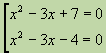
Several equations with one variable form set of equations, if the task is to find all such values of a variable, each of which is the root of at least one of these equations. A square bracket is used to indicate a population:

Equations containing a variable under the modulus sign.

The absolute value of a number A is defined as follows:

Example: Solve the equation

Solution: If

, That

. You can write it like this:

From Eq.

we find X= -9. However, with this value of the variable, the inequality does not hold, which means that the value found is not the root of this equation., That

and this equation will take the form. You can write it like this:

From Eq.

we find . The inequality is true, which means - the root of this equation.. Equations with a variable in the denominator.

Consider equations of the form

. (1)

The solution to an equation of type (1) is based on the following statement: a fraction is equal to 0 if and only if its numerator is equal to 0 and its denominator is non-zero.

In accordance with the above, the solution to the equation

is carried out in two stages: first you need to solve the equation, and then find out whether, with the found values of the variable, X denominator at 0. If q(x) ¹ 0 , then the found root of the equationis also the root of equation (1); Ifq(x) = 0, then the resulting root of the equationis also the root of equation (1). The resulting system is: Domain of the equation
f(x) = g(x) call the set of all those values of a variable X, for which the expressionf(x), and the expression g(x)make sense.

If in the process of transforming an equation its domain of definition has expanded, then extraneous roots may appear. Therefore, all found values of the variable must be checked by substitution into the original equation or using the domain of definition of the original equation.

Rational equations.

The equation

f(x) = g(x) called rational, If f(x) and g(x)-rational expressions. Moreover, if f(x) and g(x)- whole expressions, then the equation is called whole ;if at least one of the expressionsf(x), g(x)is fractional, then the rational equationf(x) = g(x) called fractional .

To solve a rational equation, you need:

find the common denominator of all available fractions;
replace this equation with a whole one, multiplying both its parts by a common denominator;
Solve the resulting whole equation;
Eliminate from its roots those that make the common denominator vanish.

Solving the equation
p(x) = 0 factorization method. p(x) can be factorized: , then the equation takes the form

. If A- root of the equation, That

, therefore at least one of the numbers

equals 0.

The opposite is also true: if X

= A- the root of at least one of the equations , , , That A- root of the equation. That is Solving equations
by introducing a new variable.

Let us explain the essence of the method with an example.

Example: Solve the equation

Solution. Let us put

, we get the equation

, where we find

. The problem comes down to solving a set of equations

The first quadratic equation has no real roots, so its discriminant is negative. From the second we find

. These are the roots of the given equation.

An equation of the form is called biquadratic

, Where A ¹ 0. The biquadratic equation is solved by introducing a new variable: putting , we arrive at the quadratic equation

. Irrational equations.
Irrational
An equation is called in which the variable is contained under the sign of the root or under the sign of raising to a fractional power. One method for solving such equations is the method of raising both sides of the equation to the same power:

A) transform the given irrational equation to the form:

;

B) we raise both sides of the resulting equation to

n-th degree:

;

B) considering that

, we get the equation

f(x) = g(x);

)We solve the equation and do a check, since raising both sides of the equation to an even power can lead to the appearance of extraneous roots. This check is carried out by substituting the found values of the variable into the original equation.

Use of site materials is possible subject to an active link.