Microsoft Excel (hereinafter simply - Excel) is a program for performing calculations and managing so-called spreadsheets.
Excel allows you to perform complex calculations that can use data located in different areas of the spreadsheet and linked together by a certain dependency. To perform such calculations in Excel, it is possible to enter various formulas into table cells. Excel performs the calculation and displays the result in the formula cell.
An important feature of using a spreadsheet is the automatic recalculation of results when cell values change. Excel can also create and update graphs based on the numbers you enter.
A cell address in spreadsheets consists of the column name followed by the row number, for example C15.
Cell addresses and signs are used to write formulas arithmetic operations(+, -, *, /, ^). The formula begins with =.
Excel provides standard functions that can be used in formulas. These are mathematical, logical, text, financial and other functions. However, in the exam you may encounter only the simplest functions: COUNT (number of non-empty cells), SUM (sum), AVERAGE (average value), MIN (minimum value), MAX (maximum value).
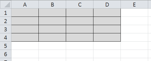
The cell range is designated as follows: A1:D4 (all cells of the rectangle from A1 to D4.
Cell addresses can be relative, absolute, or mixed.
They behave differently when copying a formula from cell to cell.
Relative addressing:
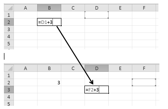
If in cell B2 we write the formula =D1+3, then the table will perceive this as “take the value of the cell two to the right and one above the current one, and add 3 to it.”
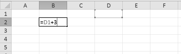
Those. address D1 is perceived by the table as a position relative to the cell where the formula is entered. This address is called relative. When copying such a formula to another cell, the table will automatically recalculate the address relative to the new location of the formula:
Absolute addressing:
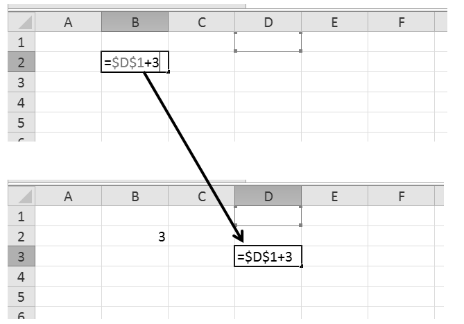
If we don’t need the address to be recalculated when copying the formula, we can “fix” it in the formula - put a $ sign in front of the letter and cell index: =$D$1+3. This address is called absolute. This formula will not change when copied:
Mixed addressing:
If we want, when copying a formula, only the cell index is automatically recalculated, for example, and the letter remains unchanged, we can “fix” only the letter in the formula (or vice versa): =$D1+3. This address is called mixed. When copying a formula, only the index in the cell address will change:

Spreadsheets. Copying formulas.
Example 1.
Cell C2 contains the formula =$E$3+D2. What form will the formula take after cell C2 is copied to cell B1?
1) =$E$3+C1 2) =$D$3+D2 3) =$E$3+E3 4) =$F$4+D2
Solution:
The location of the formula changes from C2 to B1, i.e. the formula is shifted one cell to the left and one cell up (the letter “decreases” by one and the index decreases by one). This means that all relative addresses will also change, but absolute ones (fixed with the $ sign) will remain unchanged:
=$E$3+C1.
Answer: 1
Example 2.
Cell B11 of the spreadsheet contains a formula. This formula was copied into cell A10. As a result, the value in cell A10 is calculated using the formula x-Zu, Where X- the value in cell C22, and at- value in cell D22. Indicate what formula might have been written in cell B11.
1) =C22-3*D22 2) =D$22-3*$D23 3) =C$22-3*D$22 4) =$C22-3*$D22
Solution:
Let's analyze each formula in turn:
The location of the formula changes from B11 to A10, i.e. the letter "decreases" by 1 and the index decreases by 1.
Then when copying the formulas will change as follows:
The problem conditions correspond to formula 2).
Answer: 2
Spreadsheets. Determining the meaning of a formula.
Example 3.
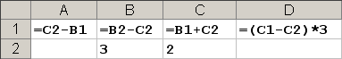
Given is a fragment of a spreadsheet:
The formula is entered in cell D1 =$A$1*B1+C2, and then copied to cell D2. What value will appear in cell D2 as a result?
1) 10 2) 14 3) 16 4) 24
Solution:
The location of the formula changes from D1 to D2, i.e. the letter does not change, but the index increases by 1.
So the formula will take the form: =$A$1*B2+C3. Let's substitute the numerical values of the cells into the formula: 1*5+9=14. The correct answer is listed at number 2.
Answer: 2
Example 4.
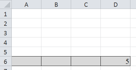
In a spreadsheet the value of a formula =AVERAGE(A6: C6) equals ( -2 ). What is the value of the formula =SUM(A6: D6) , if the value of cell D6 is 5?
1) 1 2) -1 3) -3 4) 7
Solution:
By definition of average:
AVERAGE(A6: C6) = SUM(A6:C6)/3 = -2
Means, SUM(A6:C6) = -6
SUM(A6: D6) = SUM(A6:C6)+D6 = -6+5 = -1
Answer: 2
Spreadsheets and charts.
Example 5.
A fragment of a spreadsheet in formula display mode is given.
After performing the calculations, a diagram was built using the values of the range A1:D1. Indicate the resulting diagram:

Solution:
Let's calculate the values of cells A1:D1 using formulas.
Diagram 3 corresponds to these data.
Answer: 3
Catalog of tasks.
Formula tables: setting goals
Take tests on these tasks
Return to task catalog
Version for printing and copying in MS Word
A fragment of a spreadsheet is given. A formula was copied from cell D2 to one of the cells in the range E1:E4. When copying, the cell addresses in the formula automatically changed, and the formula value became equal to 8. Which cell was the formula copied to? In your answer, indicate only one number - the number of the row in which the cell is located.
| A | B | C | D | E | |
| 1 | 1 | 2 | 3 | 4 | |
| 2 | 2 | 3 | 4 | = B$3 + $C2 | |
| 3 | 3 | 4 | 5 | 6 | |
| 4 | 4 | 5 | 6 | 7 |
Note.
Solution.
When copying a formula from cell D2, only the column number of the first term can change, and only the row number of the second term. Thus, the formulas in cells E1-E4:
E1 = C$3+$C1 = 8 E2 = C$3+$C2 = 9 E3 = C$3+$C3 = 10 E4 = C$3+$C4 = 11.
Thus, the formula was copied to cell E1.
Answer: 1.
Answer: 1
A fragment of a spreadsheet is given. A formula was copied from cell B2 to one of the cells in the range A1:A4. When copying, the cell addresses in the formula automatically changed, and the numeric value in this cell became equal to 8. Which cell was the formula copied to? In your answer, indicate only one number - the number of the row in which the cell is located.
| A | B | C | D | E | |
|---|---|---|---|---|---|
| 1 | 4 | 3 | 2 | 1 | |
| 2 | = D$3 + $C2 | 4 | 3 | 2 | |
| 3 | 6 | 5 | 4 | 3 | |
| 4 | 7 | 6 | 5 | 4 |
Note
Solution.
When copying a formula into one of the cells in the range A1:A4, the formula will take the form = C$3 + $Cn, where n is the row number of the cell into which the formula was copied. The numeric value in this cell now becomes 8, therefore, in order for the equality 5 + Cn = 8 to hold, n must be equal to 1.
Answer: 1
A fragment of a spreadsheet is given. A formula was copied from cell B2 to one of the cells in the range A1:A4. When copying, the cell addresses in the formula automatically changed, and the numeric value in this cell became equal to 13. Which cell was the formula copied to? In your answer, indicate only one number - the number of the row in which the cell is located.
| A | B | C | D | E | |
|---|---|---|---|---|---|
| 1 | 7 | 8 | 9 | 10 | |
| 2 | = D$3 + $C2 | 7 | 8 | 9 | |
| 3 | 5 | 6 | 7 | 8 | |
| 4 | 4 | 5 | 6 | 74 |
Note. The $ sign denotes absolute addressing.
Solution.
When copying a formula into one of the cells in the range A1:A4, the formula will take the form = C$3 + $Cn, where n is the row number of the cell into which the formula was copied. The numeric value in this cell now becomes 13, therefore, in order for the equality 6 + Cn = 13 to hold, n must be equal to 2.
Answer: 2
A fragment of a spreadsheet is given. A formula was copied from one of the cells in the range B1:B4 to one of the cells in the range A1:A4. At the same time, the addresses in the formula automatically changed and the numerical value in the cell where the copying was made became equal to 31. Which cell was the formula copied into? In your answer, indicate only one number - the number of the row in which the cell is located.
| A | B | C | D | E | |
|---|---|---|---|---|---|
| 1 | = D$1 + $D1 | 1 | 10 | 100 | |
| 2 | = D$2 + $D2 | 50 | 20 | 200 | |
| 3 | = D$3 + $D3 | 150 | 30 | 300 | |
| 4 | = D$4 + $D4 | 200 | 40 | 400 |
Solution.
Note that in this case, 31 can be obtained by adding the numbers in cells C1 and D3.
And since $D1 turned into $D3, we understand that the formula was copied to cell A3.
Answer: 3
A fragment of a spreadsheet is given. A formula was copied from one of the cells in the range B1:B4 to one of the cells in the range A1:A4. In this case, the addresses in the formula automatically changed and the numeric value in the cell
where the copying was made became equal to 42. Which cell was the formula copied to? In your answer, indicate only one number - the number of the row in which the cell is located.
| A | B | C | D | E | |
|---|---|---|---|---|---|
| 1 | = D$1 + $D1 | 2 | 20 | 100 | |
| 2 | = D$2 + $D2 | 52 | 40 | 200 | |
| 3 | = D$3 + $D3 | 152 | 60 | 300 | |
| 4 | = D$4 + $D4 | 252 | 80 | 400 |
Note: The $ sign denotes absolute addressing.
Solution.
The new formula will look like =C$x + $Dy, where x and y are some numbers.
Note that in this case, 42 can be obtained by adding the numbers in cells C1 and D2.
That is, the formula was copied from cell B1, since when copied, the number at C does not change due to absolute addressing.
And since $D1 turned into $D2, we understand that the formula was copied to cell A2.
Answer: 2
| A | B | C | D | E | F | |
|---|---|---|---|---|---|---|
| 1 | 300 | 20 | 10 | 41 | ||
| 2 | 400 | 200 | 100 | 42 | ||
| 3 | 500 | 2000 | 1000 | 142 | ||
| 4 | 600 | 4000 | 2000 | 242 | ||
| 5 | 700 | 6000 | 5000 | 442 | ||
| 6 | 800 | 9000 | 8000 | 842 |
In cell A3 we wrote the formula = $C2 + E$2. Cell A3 was then copied to one of the cells in column B, and the value 642 appeared in that cell. Which cell was copied to?
Note: The $ sign denotes absolute addressing.
Solution.
Note that after copying the formula from cell A3 to one of the cells B, the second term in the formula will take the form F$2. Therefore, in order for the numeric value 642 to appear in that cell after copying the formula from cell A3 to one of the cells B, the formula should look like =$C4 + F$2. To do this, you need to copy the formula from cell A3 to cell B5.
Answer: B5.
Answer: B5
Numbers are written into the cells of the spreadsheet, as shown in the figure:
| A | B | C | D | E | F | |
|---|---|---|---|---|---|---|
| 1 | 100 | 1001 | 2001 | 1001 | ||
| 2 | 200 | 2001 | 4000 | 2001 | ||
| 3 | 400 | 3001 | 6001 | 3001 | ||
| 4 | 800 | 4001 | 8000 | 4001 | ||
| 5 | 1600 | 5001 | 10001 | 5001 | ||
| 6 | 3200 | 6001 | 12000 | 6001 |
In cell A4, write the formula =$D2+E$2. Then cell A4 was copied to one of the cells in the range A1:B6, after which the numeric value 6002 appeared in that cell. Which cell was copied to?
Note: The $ sign denotes absolute addressing.
Solution.
Note that after copying the formula from cell A4 to one of the cells in the range A1:B6, the result was the sum of two terms whose last digit is one. Therefore, the formula from cell A4 was copied to one of the cells in the range B1:B6, since when copying the formula from cell A4 to one of the cells in the range A1:A6, one of the terms will be the value of cell E2, which is added to any of the other values in the table will not give the number 6002. Therefore, one of the terms is cell F2.
It remains to find the second term, which should be equal to 4001. Therefore, the other term is cell D4. To get the formula =$D4+F$2, you need to copy the formula from cell A4 to cell B6.
Answer: B6.
Answer: B6
Numbers are written into the cells of the spreadsheet, as shown in the figure:
| A | B | C | D | E | F | |
|---|---|---|---|---|---|---|
| 1 | 100 | 1001 | 2001 | 1001 | ||
| 2 | 200 | 2001 | 4000 | 2001 | ||
| 3 | 400 | 3001 | 6001 | 3001 | ||
| 4 | 800 | 4001 | 8000 | 4001 | ||
| 5 | 1600 | 5001 | 10001 | 5001 | ||
| 6 | 3200 | 6001 | 12000 | 6001 |
In cell B3 we wrote the formula =$D4+E$4. Then cell B3 was copied to one of the cells in the range A1:B6, after which the numeric value 6002 appeared in that cell. Which cell was copied to?
Note: The $ sign denotes absolute addressing.
Solution.
Note that after copying the formula from cell B3 to one of the cells in the range A1:B6, the result was the sum of two terms whose last digit is one. Therefore, the formula from cell B3 was copied to one of the cells in the range A1:A6, because when you copy the formula from cell B3 to one of the cells in the range B1:B6, one of the terms will be the value of cell E4, which is added to any of the other values in the table will not give the number 6002. Therefore, one of the terms is cell D4.
It remains to find the second term, which should be equal to 2001. Therefore, the other term is cell D2. To get the formula =$D2+D$4, you need to copy the formula from cell B3 to cell A1.
Answer: A1.
Answer: A1
Numbers are written into the cells of the spreadsheet, as shown in the figure:
| A | B | C | D | E | F | |
|---|---|---|---|---|---|---|
| 1 | 1 | 20 | 300 | 4000 | ||
| 2 | 2 | 30 | 400 | 5000 | ||
| 3 | 3 | 40 | 500 | 6000 | ||
| 4 | 4 | 50 | 600 | 7000 | ||
| 5 | 5 | 60 | 700 | 8000 | ||
| 6 | 6 | 70 | 800 | 9000 |
In cell A5, write the formula =$E3+D$4. Then cell A5 was copied to one of the cells in the range A1:B6, after which the numeric value 900 appeared in that cell. Which cell was copied to?
Note: The $ sign denotes absolute addressing.
Solution.
Note that after copying the formula from cell A5 to one of the cells in the range A1:B6, the result was the sum of the two terms, which is equal to 900. Therefore, the formula from cell A5 was copied to one of the cells in the range B1:B6, since when copying the formula from cell A5 into one of the cells of the range B1:B6, one of the terms will be the value of cell E4.
It remains to find the second term, which should be equal to 300. Therefore, the other term is cell E1. To get the formula =$E1+E$4, you need to copy the formula from cell A5 to cell B3.
Answer: B3.
Answer: B3
Numbers are written into the cells of the spreadsheet, as shown in the figure:
| A | B | C | D | E | F | |
|---|---|---|---|---|---|---|
| 1 | 1 | 20 | 300 | 4000 | ||
| 2 | 2 | 30 | 400 | 5000 | ||
| 3 | 3 | 40 | 500 | 6000 | ||
| 4 | 4 | 50 | 600 | 7000 | ||
| 5 | 5 | 60 | 700 | 8000 | ||
| 6 | 6 | 70 | 800 | 9000 |
In cell B2, write the formula =$C3+D$5. Then cell B2 was copied to one of the cells in the range A1:B6, after which the numeric value 11 appeared in that cell. Which cell was copied to?
Note: The $ sign denotes absolute addressing.
Solution.
Note that after copying the formula from cell B2 to one of the cells in the range A1:B6, the result was the sum of the two terms, which is equal to 11. Therefore, the formula from cell B2 was copied to one of the cells in the range A1:A6, since when copying the formula from cell B2 into one of the cells in the range A1:A6, one of the terms will be the value of cell C5.
It remains to find the second term, which should be equal to 6. Therefore, the other term is cell C6. To get the formula =$C6+C$5, you need to copy the formula from cell B2 to cell A5.
Answer: A5.
Answer: A5
Numbers are written into the cells of the spreadsheet, as shown in the figure:
| A | B | C | D | E | F | |
|---|---|---|---|---|---|---|
| 1 | 1 | 20 | 300 | 4000 | ||
| 2 | 2 | 30 | 400 | 5000 | ||
| 3 | 3 | 40 | 500 | 6000 | ||
| 4 | 4 | 50 | 600 | 7000 | ||
| 5 | 5 | 60 | 700 | 8000 | ||
| 6 | 6 | 70 | 800 | 9000 |
In cell A4, write the formula =$F6+E$2. Then cell A4 was copied to one of the cells in the range A1:B6, after which the numeric value 11000 appeared in that cell. Which cell was copied to?
Note: The $ sign denotes absolute addressing.
Solution.
Note that after copying the formula from cell A4 to one of the cells in the range A1:B6, the result was the sum of the two terms, which is equal to 11000. Therefore, the formula from cell A4 was copied to one of the cells in the range B1:B6, since when copying the formula from cell A4 into one of the cells in the range B1:B6, one of the terms will be the value of cell F2.
It remains to find the second term, which should be equal to 6000. Therefore, the other term is cell F3. To get the formula =$F3+F$2, you need to copy the formula from cell A4 to cell B1.
Answer: B1.
Answer: B1
Numbers are written into the cells of the spreadsheet, as shown in the figure:
| A | B | C | D | E | F | |
|---|---|---|---|---|---|---|
| 1 | 1 | 20 | 300 | 4000 | ||
| 2 | 2 | 30 | 400 | 5000 | ||
| 3 | 3 | 40 | 500 | 6000 | ||
| 4 | 4 | 50 | 600 | 7000 | ||
| 5 | 5 | 60 | 700 | 8000 | ||
| 6 | 6 | 70 | 800 | 9000 |
The formula $D5+E$1 was written in cell B3. Then cell B3 was copied to one of the cells in the range A1:B6, after which the numeric value 90 appeared in that cell. Which cell was copied to?
The lesson is devoted to how to solve task 7 of the Unified State Exam in computer science
The 7th topic - “Excel spreadsheets” - is characterized as tasks basic level complexity, execution time - approximately 3 minutes, maximum score — 1
* Some page images are taken from the presentation materials of K. Polyakov
Types of links in cells
Formulas written in table cells can be relative, absolute And mixed.
Standard Excel Functions
In the Unified State Exam, the following standard functions are found in formulas:
- COUNT - the number of non-empty cells,
- SUM - amount,
- AVERAGE - average value,
- MIN - minimum value,
- MAX - maximum value
The range of cells is indicated everywhere as a function parameter: MIN(A2:A240)
Building charts


Solving Unified State Exam (USE) tasks in computer science
Let's look at how task 7 of the Unified State Exam in computer science is solved.
Chart analysis
7_1:

Which of the diagrams correctly reflects the ratio of the total number of participants (from all three regions) for each of the test subjects?
✍ Solution:
- A bar chart allows you to determine numerical values. For example, in Tatarstan in biology the number of participants 400 and so on. Let us use it to find the total number of participants from all regions in each subject. To do this, let’s calculate the values of absolutely all columns in the diagram:
Result: 1
We suggest you take a look detailed analysis of this 7th task on video:
7_2:
The diagram shows the number of test participants by subject in different regions of Russia. 
Which of the diagrams correctly reflects the ratio of the number of history test participants in the regions?
✍ Solution:
Result: 2
For a detailed analysis of the task, watch the video:
Copying formulas
7_3: Unified State Examination in Informatics 2016, “Typical test tasks in Computer Science”, Krylova S.S., Churkina T.E. Option 2:
A fragment of a spreadsheet is given. 
From cell A3 to cell C2
C2?
✍ Solution:
Result: 180
For an analysis of this 7th task, watch the video:
7_4: Unified State Exam in Computer Science 2017, “Typical test tasks in computer science”, Krylova S.S., Churkina T.E. Option 5:
A3 to cell E2 the formula was copied. When copying, the cell addresses automatically changed.
What is the numeric value of the formula in the cell? E2?

✍ Solution:
- Consider the formula in a cell A3: = $E$1*A2 . The dollar sign means absolute addressing: when you copy a formula, the letter or number next to the dollar will not change. That is, in our case the factor $E$1 it will remain in the formula when copied.
- Since copying is carried out to the cell E2, you need to calculate how many columns to the right the formula will move: by 5 columns (from A before E). Accordingly, in the factor A2 letter A will be replaced by E.
- Now let’s calculate how many lines up the formula will shift when copying: by one (c A 3 on E 2 ). Accordingly, in the factor A2 number 2 will be replaced by 1 .
- Let's get the formula and calculate the result: =$E$1*E1 = 1
Result: 1
7_5: Task 7. Demo version of the Unified State Exam 2018 computer science:
A fragment of a spreadsheet is given. From cell B3 to cell A4 the formula was copied. When copying, the cell addresses in the formula automatically changed.
What is the numeric value of the formula in the cell? A4?
Note: The $ sign denotes absolute addressing.
✍ Solution to task 7:
- The dollar sign $ means absolute addressing:
- The $ in front of the letter means the column is fixed: i.e. when copying a formula, the column name will not change;
- The $ before the number means the line is fixed: when copying the formula, the name of the line will not change.
- In our case, the highlighted letters and numbers will not change: = $C 2+D $3
- Copying the formula one column to the left means that the letter D(in D$3) must change to the one preceding it C. When you copy a formula down one line, the value 2 (in $C2) changes to 3 .
- We get the formula:
Result: 600
For a detailed solution to this 7th task from the demo version of the Unified State Exam 2018, watch the video:
What formula was written down?
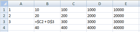
7_6: Task 7 of the Unified State Exam. Task 6 GVE grade 11 2018 (FIPI)
Kolya needs to build a table of formula values using spreadsheets 5х–3у for values X And at from 2
before 5
. To do this, first in the ranges B1:E1 And A2:A5 he wrote down the numbers from 2
before 5
. Then into the cell AT 2 wrote down the formula (A2 – x value; B1 – y value), and then copied it to all cells of the range B2:E5. As a result, I received the table presented below. 
What formula was written in the cell AT 2?
Note: The $ sign is used to indicate absolute addressing.
Options:
1)=5*$A$2–3*$B$1
2)=5*$A2–3*B$1
3)=5*A$2–3*$B1
4)=5*A2–3*$B$1
✍ Solution:
- Let's mentally imagine copying a cell with a formula separately horizontally and vertically.
- Column reference in formula A should not change the letter when copying, which means you need to put a $ sign in front of it:
Horizontally:

Vertically:

Result: 2
Meaning of SUM or AVERAGE formula
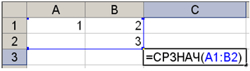
7_7: Unified State Examination in computer science task 7 (example task P-00, Polyakov K.)
Behind 
How the cell value will change C3, if after entering formulas you move the cell contents B2 V B3?
("+1" means an increase by 1
, "-1" means decrease by 1
):
Options:
1) -2
2) -1
3) 0
4) +1
✍ Solution:
- Let's analyze the spreadsheet data before moving:
- In a cell C2 there will be a number 4 , since the function CHECK Counts the number of non-empty cells in the specified range.
- In a cell C3 there will be a number 3 :
Now let's see what happens after the move:
(don't forget that the function AVERAGE doesn't count empty cells, so cell B2 not taken into account).
Result: 2
Detailed solution to the task in the video:
7_8:
In a spreadsheet, the value of the formula =AVERAGE(C2:C5) is 3 .
What is the value of the formula =SUM(C2:C4) if the cell value C5 equals 5
?
✍ Solution:
- Function AVERAGE is designed to calculate the arithmetic mean of a specified range of cells. Those. in our case, the average value of cells C2, C3, C4, C5.
- The result of the function =AVERAGE(C2:C5) is given according to the condition, let’s substitute it into the formula:
Result: 7
For a detailed solution, watch the video:
What number should be written in the cell
7_9: Unified State Examination in Informatics 2017, FIPI task option 7 (Krylov S.S., Churkina T.E.):
Given is a fragment of a spreadsheet: 
A1 so that a chart based on cell values A2:C2, matched the picture? It is known that all cell values from the considered range are non-negative.
✍ Solution:
- We have a pie chart that displays the shares of individual components in the total. Based on the image of the diagram, one can judge that, most likely, the values in all cells of the formula should be equal (the sectors of the diagram are visually equal).
- A1 -> x:
Result: 5
For a more detailed analysis, we suggest watching the video solution to this 7 Unified State Exam assignments in computer science:
Let's look at another example of solving task 7 of the Unified State Exam in computer science:
7_10: Unified State Examination in Informatics 2017 task 7 FIPI option 15 (Krylov S.S., Churkina T.E.):
Given is a fragment of a spreadsheet: 
What integer should be written in the cell C1, so that the chart constructed after performing calculations based on the values of a range of cells A2:C2 Did it match the picture?
It is known that all values of the range on which the diagram is constructed have the same sign.
✍ Solution:
- A pie chart displays the shares of individual parts in a total. In our case, the chart displays the results of formula calculations in cells A2:C2
- From the diagram you can judge that, most likely, the obtained values in the formulas in all cells should be equal (the sectors of the diagram are visually equal).
- Let's get expressions from cell formulas by substituting C1 -> x:
For effective preparation in computer science, brief theoretical material for completing the task is given for each task. Over 10 training tasks with analysis and answers have been selected, developed based on the demo version of previous years.
There are no changes to the 2019 Unified State Exam KIM in computer science and ICT.
Areas in which knowledge will be tested:
- Programming;
- Algorithmization;
- ICT tools;
- Information activities;
- Information processes.
Necessary actions when preparation:
- Repetition of the theoretical course;
- Solution tests in computer science online;
- Knowledge of programming languages;
- Improve mathematics and mathematical logic;
- Use a wider range of literature – school curriculum is not enough for success on the Unified State Exam.
Exam structure
The duration of the exam is 3 hours 55 minutes (255 minutes), an hour and a half of which is recommended to be devoted to completing the tasks of the first part of the KIMs.
The tasks in the tickets are divided into blocks:
- Part 1- 23 tasks with short answer.
- Part 2- 4 tasks with detailed answers.
Of the proposed 23 tasks of the first part exam paper 12 refer to the basic level of knowledge testing, 10 – increased complexity, 1 – high level of complexity. Three problems of the second part high level complexity, one – increased.
When making a decision, it is necessary to record a detailed answer (free form).
In some tasks, the text of the condition is presented in five programming languages at once - for the convenience of students.
Points for computer science assignments
1 point - for 1-23 tasks
2 points - 25.
3 points - 24, 26.
4 points - 27.
Total: 35 points.
For admission to technical university intermediate level, you must score at least 62 points. To enter the capital's university, the number of points must correspond to 85-95.
To successfully write an examination paper, a clear knowledge of theory and constant practice in solving tasks.
Your formula for success
Work + work on mistakes + carefully read the question from beginning to end to avoid mistakes = maximum score on the Unified State Exam in computer science.
Analysis of task 7 of the Unified State Exam 2017 in computer science from the demo version project. This is a task of a basic level of difficulty. Approximate time to complete the task is 3 minutes.
Content elements tested: knowledge of technology for processing information in spreadsheets and methods of visualizing data using charts and graphs. Content elements tested on the Unified State Exam: Mathematical processing of statistical data. Using tools for solving statistical and computational-graphical problems.
Task 7:
A fragment of a spreadsheet is given. A formula was copied from cell A2 to cell B3. When copying, the cell addresses in the formula automatically changed. Write down the numerical value of the formula in cell B3 in your answer.
Note: The $ sign denotes absolute addressing.
Answer: ________
Our formula =C$2+D$3 in a cell A2 contains two mixed links.
- in the first C$2- the address of line 2 does not change when copying
- in the second D$3- the address of line 3 does not change when copying
Our formula =C$2+D$3 was copied from a cell A2 to cell B3.
— moved one column to the right (increased by one column)
— moved one line down (increased by one line)
Therefore, after copying the formula =C$2+D$3, will take the form =D$2+E$3.

Evaluating this expression gives the following result: 70+5=75 .