Calculation of relative error formula. Absolute and relative measurement errors

X = X avg X

Absolute

error

Relative

error

a+ b

a+ b

When measuring any quantity, there is invariably some deviation from the true value, due to the fact that no instrument can give an accurate result. In order to determine the permissible deviations of the obtained data from the exact value, the representations of relative and unconditional errors are used.

You will need

• – measurement results;
• - calculator.

Instructions

1. First of all, take several measurements with an instrument of the same value in order to have a chance of calculating the actual value. The more measurements are taken, the more accurate the result will be. Let's say weigh an apple on an electronic scale. It is possible that you got results of 0.106, 0.111, 0.098 kg.

2. Now calculate the actual value of the quantity (real, because it is impossible to detect the true one). To do this, add up the resulting totals and divide them by the number of measurements, that is, find the arithmetic mean. In the example, the actual value would be (0.106+0.111+0.098)/3=0.105.

3. To calculate the unconditional error of the first measurement, subtract the actual value from the total: 0.106-0.105=0.001. In the same way, calculate the unconditional errors of the remaining measurements. Please note that regardless of whether the result turns out to be a minus or a plus, the sign of the error is invariably positive (that is, you take the absolute value).

4. In order to obtain the relative error of the first measurement, divide the unconditional error by the actual value: 0.001/0.105=0.0095. Please note that the relative error is usually measured as a percentage, therefore multiply the resulting number by 100%: 0.0095x100% = 0.95%. In the same way, calculate the relative errors of other measurements.

5. If the true value is already known, immediately begin calculating the errors, eliminating the search for the arithmetic mean of the measurement results. Immediately subtract the resulting total from the true value, and you will discover an unconditional error.

6. After this, divide the absolute error by the true value and multiply by 100% - this will be the relative error. Let's say the number of students is 197, but it was rounded to 200. In this case, calculate the rounding error: 197-200=3, relative error: 3/197x100%=1.5%.

Error is a value that determines the permissible deviations of the obtained data from the exact value. There are concepts of relative and unconditional error. Finding them is one of the tasks of a mathematical review. However, in practice, it is more important to calculate the error in the spread of some measured indicator. Physical devices have their own possible errors. But it’s not the only thing that needs to be considered when determining the indicator. To calculate the scatter error σ, it is necessary to carry out several measurements of this quantity.

You will need

• Device for measuring the required value

Instructions

1. Measure the value you need with a device or other measuring device. Repeat measurements several times. The larger the values ​​obtained, the higher the accuracy of determining the scatter error. Traditionally, 6-10 measurements are taken. Write down the resulting set of measured value values.

2. If all the obtained values ​​are equal, therefore, the scatter error is zero. If there are different values ​​in the series, calculate the error of scatter. There is a special formula to determine it.

3. According to the formula, first calculate the average value<х>from the obtained values. To do this, add up all the values ​​and divide their sum by the number of measurements taken n.

4. Determine one by one the difference between the entire value obtained and the average value<х>. Write down the results of the differences obtained. After this, square all the differences. Find the sum of the given squares. You will save the final total amount received.

5. Evaluate the expression n(n-1), where n is the number of measurements you take. Divide the total from the previous calculation by the resulting value.

6. Take the square root of the quotient of the division. This will be the error in the spread of σ, the value you measured.

When carrying out measurements, it is impossible to guarantee their accuracy; every device gives a certain error. In order to find out the measurement accuracy or the accuracy class of the device, you need to determine the unconditional and relative error .

You will need

• – several measurement results or another sample;
• - calculator.

Instructions

1. Take measurements at least 3-5 times to be able to calculate the actual value of the parameter. Add up the resulting results and divide them by the number of measurements, you get the real value, which is used in tasks instead of the true one (it is impossible to determine it). Let's say, if the measurements gave a total of 8, 9, 8, 7, 10, then the actual value will be equal to (8+9+8+7+10)/5=8.4.

2. Discover unconditional error of the entire measurement. To do this, subtract the actual value from the measurement result, neglecting the signs. You will receive 5 unconditional errors, one for each measurement. In the example they will be equal to 8-8.4 = 0.4, 9-8.4 = 0.6, 8-8.4 = 0.4, 7-8.4 = 1.4, 10-8.4 =1.6 (total modules taken).

3. To find out the relative error any dimension, divide the unconditional error to the actual (true) value. After this, multiply the resulting total by 100%; traditionally this value is measured as a percentage. In the example, discover the relative error thus: ?1=0.4/8.4=0.048 (or 4.8%), ?2=0.6/8.4=0.071 (or 7.1%), ?3=0.4/ 8.4=0.048 (or 4.8%), ?4=1.4/8.4=0.167 (or 16.7%), ?5=1.6/8.4=0.19 (or 19 %).

4. In practice, to display the error particularly accurately, the standard deviation is used. In order to detect it, square all the unconditional measurement errors and add them together. Then divide this number by (N-1), where N is the number of measurements. By calculating the root of the resulting total, you will obtain the standard deviation, which characterizes error measurements.

5. In order to discover the ultimate unconditional error, find the minimum number that is obviously greater than the unconditional error or equal to it. In the example considered, simply select the largest value - 1.6. It is also occasionally necessary to discover the limiting relative error, in this case, find a number greater than or equal to the relative error, in the example it is 19%.

An inseparable part of any measurement is some error. It represents a good review of the accuracy of the research conducted. According to the form of presentation, it can be unconditional and relative.

You will need

• - calculator.

Instructions

1. Errors in physical measurements are divided into systematic, random and impudent. The former are caused by factors that act identically when measurements are repeated many times. They are continuous or change regularly. They can be caused by incorrect installation of the device or imperfection of the chosen measurement method.

2. The second appear from the power of causes, and causeless disposition. These include incorrect rounding when calculating readings and the power of the environment. If such errors are much smaller than the scale divisions of this measuring device, then it is appropriate to take half the division as the absolute error.

3. Miss or daring error represents the result of tracking, one that is sharply different from all the others.

4. Unconditional error approximate numerical value is the difference between the result obtained during the measurement and the true value of the measured value. The true or actual value especially accurately reflects the physical quantity being studied. This error is the easiest quantitative measure of error. It can be calculated using the following formula: ?Х = Hisl – Hist. It can take on positive and negative meanings. For a better understanding, let's look at an example. The school has 1205 students, when rounded to 1200 the absolute error equals: ? = 1200 – 1205 = 5.

5. There are certain rules for calculating the error of values. Firstly, unconditional error the sum of 2 independent quantities is equal to the sum of their unconditional errors: ?(X+Y) = ?X+?Y. A similar approach is applicable for the difference of 2 errors. You can use the formula: ?(X-Y) = ?X+?Y.

6. The amendment constitutes an unconditional error, taken with the opposite sign: ?п = -?. It is used to eliminate systematic errors.

Measurements physical quantities are invariably accompanied by one or another error. It represents the deviation of the measurement results from the true value of the measured value.

You will need

• -measuring device:
• -calculator.

Instructions

1. Errors may arise as a result of the power of various factors. Among them, we can highlight the imperfection of measurement tools or methods, inaccuracies in their manufacture, and failure to comply with special conditions when conducting surveys.

2. There are several systematizations of errors. According to the form of presentation, they can be unconditional, relative and reduced. The first represent the difference between the calculated and actual value of a quantity. They are expressed in units of the phenomenon being measured and are found using the formula:?x = hisl-hist. The latter are determined by the ratio of unconditional errors to the true value of the indicator. The calculation formula has the form:? = ?x/hist. It is measured in percentages or shares.

3. The reduced error of the measuring device is found as the ratio?x to the normalizing value xn. Depending on the type of device, it is taken either equal to the measurement limit or assigned to a certain range.

4. According to the conditions of origin, they distinguish between basic and additional. If the measurements were carried out under typical conditions, then the 1st type appears. Deviations caused by values ​​outside the typical range are additional. To evaluate it, the documentation usually establishes standards within which the value can change if the measurement conditions are violated.

5. Also, errors in physical measurements are divided into systematic, random and daring. The first are caused by factors that act when measurements are repeated many times. The second appear from the power of causes, and causeless disposition. A miss represents the outcome of tracking, the one that is radically different from all the others.

6. Depending on the nature of the quantity being measured, different methods for measuring error can be used. The first of them is the Kornfeld method. It is based on calculating the confidence interval ranging from the smallest to the maximum total. The error in this case will be half the difference between these totals: ?x = (xmax-xmin)/2. Another method is the calculation of the mean square error.

Measurements can be taken with varying degrees of accuracy. At the same time, even precision instruments are not absolutely accurate. The absolute and relative errors may be small, but in reality they are virtually unchanged. The difference between the approximate and exact values ​​of a certain quantity is called unconditional error. In this case, the deviation can be either large or small.

You will need

• – measurement data;
• - calculator.

Instructions

1. Before calculating the unconditional error, take several postulates as initial data. Eliminate daring errors. Assume that the necessary corrections have already been calculated and included in the total. Such an amendment could be, say, moving the starting point of measurements.

2. Take as an initial position that random errors are known and taken into account. This implies that they are smaller than the systematic ones, that is, unconditional and relative, characteristic of this particular device.

3. Random errors affect the outcome of even highly accurate measurements. Consequently, every result will be more or less close to the unconditional, but there will invariably be discrepancies. Determine this interval. It can be expressed by the formula (Xism-?X)?Xism? (Hism+?X).

4. Determine the value that is as close as possible to the true value. In real measurements, the arithmetic mean is taken, which can be determined using the formula shown in the figure. Take the total as the true value. In many cases, the reading of the reference instrument is accepted as accurate.

5. Knowing the true measurement value, you can detect an unconditional error that must be considered in all subsequent measurements. Find the value of X1 - the data of a certain measurement. Determine the difference?X by subtracting the smaller number from the larger number. When determining the error, only the modulus of this difference is taken into account.

Note!
As usual, in practice it is impossible to carry out an absolutely accurate measurement. Consequently, the maximum error is taken as the reference value. It represents the highest value of the absolute error module.

Helpful advice
In utilitarian measurements, the value of the unconditional error is usually taken to be half the smallest division value. When working with numbers, the unconditional error is taken to be half the value of the digit, which is located in the next digit after the exact digits. To determine the accuracy class of an instrument, the most important thing is the ratio of the absolute error to the total measurement or to the length of the scale.

Measurement errors are associated with imperfection of instruments, instruments, and methodology. Accuracy also depends on the observation and state of the experimenter. Errors are divided into unconditional, relative and reduced.

Instructions

1. Let a single measurement of a quantity give the result x. The true value is denoted by x0. Then unconditional error?x=|x-x0|. It estimates the unconditional measurement error. Unconditional error consists of 3 components: random errors, systematic errors and misses. Usually, when measuring with an instrument, half the division value is taken as an error. For a millimeter ruler this would be 0.5 mm.

2. The true value of the measured value is in the interval (x-?x; x+?x). In short, this is written as x0=x±?x. The main thing is to measure x and ?x in the same units and write the numbers in the same format, say the whole part and three digits after the decimal point. It turns out unconditional error gives the boundaries of the interval in which, with some probability, the true value is located.

3. Relative error expresses the ratio of the unconditional error to the actual value of the quantity: ?(x)=?x/x0. This is a dimensionless quantity and can also be written as a percentage.

4. Measurements can be direct or indirect. In direct measurements, the desired value is immediately measured with the appropriate device. Let's say the length of a body is measured with a ruler, the voltage with a voltmeter. In indirect measurements, a value is found using the formula for the relationship between it and the measured values.

5. If the result is a connection between 3 easily measured quantities that have errors?x1, ?x2, ?x3, then error indirect measurement?F=?[(?x1 ?F/?x1)?+(?x2 ?F/?x2)?+(?x3 ?F/?x3)?]. Here?F/?x(i) are the partial derivatives of the function with respect to any of the easily measured quantities.

Helpful advice
Errors are daring inaccuracies in measurements that occur due to malfunction of instruments, inattentiveness of the experimenter, or violation of the experimental methodology. In order to reduce the likelihood of such mistakes, when taking measurements, be careful and describe the results obtained in detail.

The result of any measurement is inevitably accompanied by a deviation from the true value. The measurement error can be calculated using several methods depending on its type, for example, statistical methods for determining the confidence interval, standard deviation, etc.

Instructions

1. There are several reasons why errors measurements. These are instrument inaccuracy, imperfect methodology, as well as errors caused by the inattention of the operator taking measurements. In addition, the true value of a parameter is often taken to be its actual value, which in fact is only particularly possible, based on a review of a statistical sample of the results of a series of experiments.

2. Error is a measure of the deviation of a measured parameter from its true value. According to Kornfeld's method, a confidence interval is determined, one that guarantees a certain degree of security. In this case, the so-called confidence limits are found within which the value fluctuates, and the error is calculated as the half-sum of these values:? = (xmax – xmin)/2.

3. This is an interval estimate errors, which makes sense to carry out with a small statistical sample size. A point estimate consists of calculating the mathematical expectation and standard deviation.

4. The mathematical expectation is the integral sum of a series of products of 2 tracking parameters. These are, in fact, the values ​​of the measured quantity and its probability at these points: M = ?xi pi.

5. The classic formula for calculating the standard deviation involves calculating the average value of the analyzed sequence of values ​​of the measured value, and also considers the volume of a series of experiments performed:? = ?(?(xi – xav)?/(n – 1)).

6. According to the method of expression, unconditional, relative and reduced errors are also distinguished. The unconditional error is expressed in the same units as the measured value and is equal to the difference between its calculated and true value:?x = x1 – x0.

7. The relative measurement error is related to the unconditional error, but is more highly effective. It has no dimension and is sometimes expressed as a percentage. Its value is equal to the ratio of the unconditional errors to the true or calculated value of the measured parameter:?x = ?x/x0 or?x = ?x/x1.

8. The reduced error is expressed by the relationship between the unconditional error and some conventionally accepted value x, which is constant for all measurements and is determined by the calibration of the instrument scale. If the scale starts from zero (one-sided), then this normalizing value is equal to its upper limit, and if it is two-sided, it is equal to the width of each of its ranges:? = ?x/xn.

Self-monitoring for diabetes is considered an important component of treatment. A glucometer is used to measure blood sugar at home. The possible error of this device is higher than that of laboratory glycemic analyzers.

Measuring blood sugar is necessary to assess the effectiveness of diabetes treatment and to adjust the dose of medications. How many times a month you will need to measure your sugar depends on the prescribed therapy. Occasionally, blood sampling for review is necessary several times during the day, sometimes 1-2 times a week is enough. Self-monitoring is especially necessary for pregnant women and patients with type 1 diabetes.

Permissible error for a glucometer according to international standards

The glucometer is not considered a high-precision device. It is intended only for the approximate determination of blood sugar concentration. The possible error of a glucometer according to world standards is 20% when glycemia is more than 4.2 mmol/l. Let's say, if during self-control a sugar level of 5 mmol/l is recorded, then the real concentration value is in the range from 4 to 6 mmol/l. The possible error of a glucometer under standard conditions is measured as a percentage, not in mmol/l. The higher the indicators, the larger the error in absolute numbers. Let's say, if blood sugar reaches about 10 mmol/l, then the error does not exceed 2 mmol/l, and if sugar is about 20 mmol/l, then the difference with the result of the laboratory measurement can be up to 4 mmol/l. In most cases, the glucometer overestimates glycemic levels. The standards allow the stated measurement error to be exceeded in 5% of cases. This means that every twentieth study can significantly distort the results.

Permissible error for glucometers from various companies

Glucometers are subject to mandatory certification. The documents accompanying the device usually indicate figures for the possible measurement error. If this item is not in the instructions, then the error corresponds to 20%. Some glucometer manufacturers place special emphasis on measurement accuracy. There are devices from European companies that have a possible error of less than 20%. The best figure today is 10-15%.

Error in the glucometer during self-monitoring

The permissible measurement error characterizes the operation of the device. Several other factors also affect the accuracy of the survey. Abnormally prepared skin, too small or too much volume of a drop of blood received, unacceptable temperature conditions - all this can lead to errors. Only if all the rules of self-control are followed, can one rely on the stated possible research error. You can learn the rules of self-monitoring with the help of a glucometer from your doctor. The accuracy of the glucometer can be checked at a service center. Manufacturers' warranties include free consultation and troubleshooting.

Errors in measurements of physical quantities

1.Introduction(measurement and measurement error)

2.Random and systematic errors

3.Absolute and relative errors

4. Errors of measuring instruments

5. Accuracy class of electrical measuring instruments

6.Reading error

7.Total absolute error of direct measurements

8.Recording the final result of direct measurement

9. Errors of indirect measurements

10.Example

1. Introduction(measurement and measurement error)

Physics as a science was born more than 300 years ago, when Galileo essentially created the scientific study of physical phenomena: physical laws are established and tested experimentally by accumulating and comparing experimental data, represented by a set of numbers, laws are formulated in the language of mathematics, i.e. using formulas that connect numerical values ​​of physical quantities by functional dependence. Therefore, physics is an experimental science, physics is a quantitative science.

Let's get acquainted with some characteristic features of any measurements.

Measurement is finding the numerical value of a physical quantity experimentally using measuring instruments (ruler, voltmeter, watch, etc.).

Measurements can be direct or indirect.

Direct measurement is finding the numerical value of a physical quantity directly by means of measurement. For example, length - with a ruler, atmospheric pressure - with a barometer.

Indirect measurement is finding the numerical value of a physical quantity using a formula that connects the desired quantity with other quantities determined by direct measurements. For example, the resistance of a conductor is determined by the formula R=U/I, where U and I are measured by electrical measuring instruments.

Let's look at an example of measurement.

Measure the length of the bar with a ruler (division value is 1 mm). We can only say that the length of the bar is between 22 and 23 mm. The width of the interval of “unknown” is 1 mm, that is, equal to the division price. Replacing the ruler with a more sensitive device, such as a caliper, will reduce this interval, which will lead to increased measurement accuracy. In our example, the measurement accuracy does not exceed 1mm.

Therefore, measurements can never be made absolutely accurately. The result of any measurement is approximate. Uncertainty in measurement is characterized by error - the deviation of the measured value of a physical quantity from its true value.

Let us list some of the reasons leading to errors.

1. Limited manufacturing accuracy of measuring instruments.

2. Influence on the measurement of external conditions (temperature changes, voltage fluctuations...).

3. Actions of the experimenter (delay in starting the stopwatch, different eye positions...).

4. The approximate nature of the laws used to find measured quantities.

The listed causes of errors cannot be eliminated, although they can be minimized. To establish the reliability of conclusions obtained as a result of scientific research, there are methods for assessing these errors.

2. Random and systematic errors

Errors arising during measurements are divided into systematic and random.

Systematic errors are errors corresponding to the deviation of the measured value from the true value of a physical quantity, always in one direction (increase or decrease). With repeated measurements, the error remains the same.

Reasons for systematic errors:

1) non-compliance of measuring instruments with the standard;

2) incorrect installation of measuring instruments (tilt, imbalance);

3) discrepancy between the initial indicators of the instruments and zero and ignoring the corrections that arise in connection with this;

4) discrepancy between the measured object and the assumption about its properties (presence of voids, etc.).

Random errors are errors that change their numerical value in an unpredictable way. Such errors are caused by a large number of uncontrollable reasons that affect the measurement process (irregularities on the surface of the object, wind blowing, power surges, etc.). The influence of random errors can be reduced by repeating the experiment many times.

3. Absolute and relative errors

To quantify the quality of measurements, the concepts of absolute and relative measurement errors are introduced.

As already mentioned, any measurement gives only an approximate value of a physical quantity, but you can specify an interval that contains its true value:

A pr - D A< А ист < А пр + D А

Value D A is called the absolute error in measuring the quantity A. The absolute error is expressed in units of the quantity being measured. The absolute error is equal to the modulus of the maximum possible deviation of the value of a physical quantity from the measured value. And pr is the value of a physical quantity obtained experimentally; if the measurement was carried out repeatedly, then the arithmetic mean of these measurements.

But to assess the quality of measurement it is necessary to determine the relative error e. e = D A/A pr or e= (D A/A pr)*100%.

If a relative error of more than 10% is obtained during a measurement, then they say that only an estimate of the measured value has been made. In physics workshop laboratories, it is recommended to carry out measurements with a relative error of up to 10%. In scientific laboratories, some precise measurements (for example, determining the wavelength of light) are performed with an accuracy of millionths of a percent.

4. Errors of measuring instruments

These errors are also called instrumental or instrumental. They are determined by the design of the measuring device, the accuracy of its manufacture and calibration. Usually they are content with the permissible instrumental errors reported by the manufacturer in the passport for this device. These permissible errors are regulated by GOSTs. This also applies to standards. Usually the absolute instrumental error is denoted D and A.

If there is no information about the permissible error (for example, with a ruler), then half the division value can be taken as this error.

When weighing, the absolute instrumental error consists of the instrumental errors of the scales and weights. The table shows the most common permissible errors

measuring instruments encountered in school experiments.

5. Accuracy class of electrical measuring instruments

Pointer electrical measuring instruments, based on permissible error values, are divided into accuracy classes, which are indicated on the instrument scales with the numbers 0.1; 0.2; 0.5; 1.0; 1.5; 2.5; 4.0. Accuracy class g pr The device shows what percentage the absolute error is from the entire scale of the device.

g pr = (D and A/A max)*100% .

For example, the absolute instrumental error of a class 2.5 device is 2.5% of its scale.

If the accuracy class of the device and its scale are known, then the absolute instrumental measurement error can be determined

D and A = (g pr * A max)/100.

To increase the accuracy of measurements with a pointer electrical measuring instrument, it is necessary to select a device with such a scale that during the measurement process it is located in the second half of the instrument scale.

6. Reading error

The reading error results from insufficiently accurate readings of the measuring instruments.

In most cases, the absolute reading error is taken equal to half the division value. Exceptions are made when measuring with a clock (the hands move jerkily).

The absolute error of reading is usually denoted D oA

7. Total absolute error of direct measurements

When performing direct measurements of physical quantity A, the following errors must be assessed: D and A, D oA and D сА (random). Of course, other sources of errors associated with incorrect installation of instruments, misalignment of the initial position of the instrument arrow with 0, etc. should be excluded.

The total absolute error of direct measurement must include all three types of errors.

If the random error is small compared to the smallest value that can be measured by a given measuring instrument (compared to the division value), then it can be neglected and then one measurement is sufficient to determine the value of a physical quantity. Otherwise, probability theory recommends finding the measurement result as the arithmetic mean value of the results of the entire series of multiple measurements, and calculating the error of the result using the method of mathematical statistics. Knowledge of these methods goes beyond the school curriculum.

8. Recording the final result of direct measurement

The final result of measuring the physical quantity A should be written in this form;

A=A pr + D A, e= (D A/A pr)*100%.

And pr is the value of a physical quantity obtained experimentally; if the measurement was carried out repeatedly, then the arithmetic mean of these measurements. D A is the total absolute error of direct measurement.

Absolute error is usually expressed in one significant figure.

Example: L=(7.9 + 0.1) mm, e=13%.

9. Errors of indirect measurements

When processing the results of indirect measurements of a physical quantity that is functionally related to physical quantities A, B and C, which are measured directly, the relative error of the indirect measurement is first determined e=D X/X pr, using the formulas given in the table (without evidence).

The absolute error is determined by the formula D X=X pr *e,

where e expressed as a decimal fraction rather than a percentage.

The final result is recorded in the same way as in the case of direct measurements.

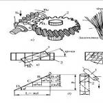
Example: Let's calculate the error in measuring the friction coefficient using a dynamometer. The experiment consists of pulling a block evenly over a horizontal surface and measuring the applied force: it is equal to the sliding friction force.

Using a dynamometer, weigh the block with weights: 1.8 N. F tr =0.6 N

μ = 0.33. The instrumental error of the dynamometer (we find it from the table) is Δ and = 0.05 N, Reading error (half the division value)

Δ o =0.05 N. The absolute error in measuring weight and friction force is 0.1 N.

Relative measurement error (5th line in the table)

, therefore the absolute error of indirect measurement μ is 0.22*0.33=0.074

In the practical implementation of the measurement process, regardless of the accuracy of the measuring instruments, the correctness of the methodology and thoroughness
When performing measurements, the measurement results differ from the true value of the measured value, i.e. measurement errors are inevitable. When assessing the error, the real value is taken instead of the true value; therefore, only an approximate estimate of the measurement error can be given. Assessment of the reliability of the measurement result, i.e. determining measurement error is one of the main tasks of metrology.
Error is the deviation of a measurement result from the true value of the measured value. Errors can be roughly divided into errors of measuring instruments and errors of measurement results.
Errors of measuring instruments were discussed in Chapter 3.
Measurement result error is a number indicating the possible limits of uncertainty in the value of the measured quantity.
Below we will give a classification and consider the errors of the measurement results.
By numerical expression method differentiate absolute and relative errors.
Depending on the source of occurrence there are errors instrumental, methodological, counting and installations.
According to the patterns of manifestation measurement errors are divided by systematic, progressive, random and gross.
Let us consider these measurement errors in more detail.

4.1. Absolute and relative errors

Absolute error D is the difference between the measured X and the true X and the values ​​of the measured quantity. The absolute error is expressed in units of the measured value: D = X - Chi.
Since the true value of the measured quantity cannot be determined, in practice the actual value of the measured quantity Xd is used instead. The actual value is found experimentally, by using fairly accurate methods and measuring instruments. It differs little from the true value and can be used instead to solve the problem. During verification, the readings of standard measuring instruments are usually taken as the actual value. Thus, in practice, the absolute error is found using the formula D » X - Xd. Relative error d is the ratio of the absolute measurement error to the true (actual) value of the measured quantity (it is usually expressed as a percentage): .

4.2. Instrumental and methodological errors,
counting and setting

Instrumental(instrumental or instrumental) errors are those that belong to a given measuring instrument, can be determined during its tests and are entered in its passport.
These errors are due to design and technological shortcomings of measuring instruments, as well as the result of their wear, aging or malfunction. Instrumental errors, caused by the errors of the measuring instruments used, were discussed in Chapter 3.
However, in addition to instrumental errors, during measurements there are also errors that cannot be attributed to a given device, cannot be indicated in its passport and are called methodical, those. associated not with the device itself, but with the method of its use.
Methodological errors may arise due to imperfect development of the theory of phenomena underlying the measurement method, inaccuracy of the relationships used to find an estimate of the measured value, as well as due to the discrepancy between the measured value and its model.
Let's consider examples illustrating the methodological measurement error.
The object of study is an alternating voltage source, the amplitude value of which Um need to be measured. Based on a preliminary study of the research object, a sinusoidal voltage generator was adopted as its model. Using a voltmeter designed for measuring the effective values ​​of alternating voltages, and knowing the relationship between the effective and amplitude values ​​of the sinusoidal voltage, we obtain the measurement result in the form Um = × Uv, Where UV- voltmeter reading. A more thorough study of the object could reveal that the shape of the measured voltage differs from sinusoidal and a more correct relationship between the value of the measured quantity and the voltmeter reading Um =k× UV, Where k¹ . Thus, the imperfection of the adopted model of the research object leads to a methodological measurement error DU = × UV-k× Uv.
This error can be reduced either by calculating the value k based on an analysis of the shape of the measured voltage curve, or by replacing the measuring instrument by taking a voltmeter designed for measuring the amplitude values ​​of alternating voltages.
A very common reason for the occurrence of methodological errors is the fact that, when organizing measurements, we are forced to measure (or consciously measure) not the value that should be measured, but some other value that is close, but not equal to it.

An example of such a methodological error is the error in measuring voltage with a voltmeter with a finite resistance (Fig. 4.1).
Due to the voltmeter shunting the section of the circuit on which the voltage is measured, it turns out to be less than it was before connecting the voltmeter. Indeed, the voltage that the voltmeter will show is determined by the expression U = I×Rv. Considering that the current in the circuit I =E/(Ri +Rv), That
< .
Therefore, for the same voltmeter, connected alternately to different sections of the circuit under study, this error is different: in low-resistance sections it is negligible, but in high-resistance sections it can be very large. This error could be eliminated if the voltmeter were constantly connected to this section of the circuit for the entire time the device is operating (as on a power plant switchboard), but this is unprofitable for many reasons.
There are often cases when it is generally difficult to indicate a measurement method that excludes methodological error. Let, for example, the temperature of the hot ingots coming from the furnace to the rolling mill be measured. The question is, where to place the temperature sensor (for example, a thermocouple): under the blank, on the side or above the blank? Wherever we place it, we will not measure the internal temperature of the body of the blank, i.e. we will have a significant methodological error, since we are measuring not what is needed, but what is simpler (it is not possible to drill a channel in each blank to place a thermocouple in its center).
Thus, the main distinctive feature of methodological errors is the fact that they cannot be indicated in the instrument’s passport, but must be assessed by the experimenter himself when organizing the chosen measurement technique, therefore he must clearly distinguish between the actual measurable they are the size of subject to measurement.
Reading error occurs due to insufficiently accurate readings. It is due to the subjective characteristics of the observer (for example, interpolation error, i.e. inaccurate reading of division fractions on the instrument scale) and the type of reading device (for example, parallax error). There are no reading errors when using digital measuring instruments, which is one of the reasons for the prospects of the latter.
Installation error caused by deviation of measurement conditions from normal, i.e. conditions under which calibration and verification of measuring instruments were carried out. This includes, for example, errors from incorrect installation of the device in space or its pointer to the zero mark, from changes in temperature, supply voltage and other influencing quantities.
The types of errors considered are equally suitable for characterizing the accuracy of both individual measurement results and measuring instruments.

4.3. Systematic, progressive, random and gross errors

Systematic measurement error Dc is a component of the measurement error that remains constant or changes naturally with repeated measurements of the same quantity.
The causes of systematic errors can usually be established during the preparation and conduct of measurements. These reasons are very diverse: imperfection of the measuring instruments and methods used, incorrect installation of the measuring instrument, the influence of external factors (influencing quantities) on the parameters of the measuring instruments and on the measurement object itself, shortcomings of the measurement method (methodological errors), individual characteristics of the operator (subjective errors) and etc. According to the nature of their manifestation, systematic errors are divided into constant and variable. Constants include, for example, errors caused by inaccurate adjustment of the measure value, incorrect calibration of the instrument scale, incorrect installation of the instrument relative to the direction of magnetic fields, etc. Variable systematic errors are caused by the influence of influencing quantities on the measurement process and can arise, for example, when changing the voltage of the device's power supply, external magnetic fields, the frequency of the measured alternating voltage, etc. The main feature of systematic errors is that their dependence on the influencing quantities is subject to a certain law. This law can be studied, and the measurement result can be clarified by introducing amendments if the numerical values ​​of these errors are determined. Another way to reduce the influence of systematic errors is to use measurement methods that make it possible to eliminate the influence of systematic errors without determining their values ​​(for example, the substitution method).
The result of measurements is the closer to the true value of the measured value, the smaller the remaining non-excluded systematic errors. The presence of excluded systematic errors determines the accuracy of measurements, quality reflecting the closeness to zero of systematic errors. The measurement result will be as correct as it is undistorted by systematic errors, and the smaller these errors, the more correct it is.
Progressive(or drift) are unpredictable errors that change slowly over time. These errors, as a rule, are caused by the aging processes of certain parts of the equipment (discharge of power supplies, aging of resistors, capacitors, deformation of mechanical parts, shrinkage of paper tape in recorders, etc.). A feature of progressive errors is that they can be corrected by introducing an amendment only at a given point in time, and then increase again unpredictably. Therefore, unlike systematic errors, which can be corrected by a correction found once for the entire service life of the device, progressive errors require continuous repetition of the correction and the more often, the smaller their residual value should be. Another feature of progressive errors is that their change over time is a non-stationary random process and therefore, within the framework of a well-developed theory of stationary random processes, they can be described only with reservations.
Random measurement error— component of the measurement error that changes randomly during repeated measurements of the same quantity. The value and sign of random errors cannot be determined; they cannot be directly taken into account due to their chaotic changes caused by the simultaneous influence of various factors independent of each other on the measurement result. Random errors are detected during repeated measurements of the same quantity (individual measurements in this case are called observations) using the same measuring instruments under the same conditions by the same observer, i.e. for equal-precision (equidispersed) measurements. The influence of random errors on the measurement result is taken into account by the methods of mathematical statistics and probability theory.
Gross measurement errors - random measurement errors that significantly exceed the errors expected under given conditions.
Gross errors (misses) are usually caused by incorrect readings from the instrument, an error in recording observations, the presence of a strongly influencing quantity, malfunction of measuring instruments and other reasons. As a rule, measurement results containing gross errors are not taken into account, so gross errors have little effect on the accuracy of the measurement. It is not always easy to detect a mistake, especially with a single measurement; It is often difficult to distinguish a gross error from a large random error. If gross errors occur frequently, we will question all measurement results. Therefore, gross errors affect the validity of measurements.
In conclusion of the described division of errors of instruments and measurement results into random, progressive and systematic components, it is necessary to pay attention to the fact that such division is a very simplified method of their analysis. Therefore, one should always remember that in reality, these error components appear together and form a single non-stationary random process. The error of the measurement result can be represented in the form of the sum of random and systematic errors Dс: D = Dс +. The measurement errors include a random component, so it should be considered a random variable.
Consideration of the nature of the manifestation of measurement errors shows us that the only correct way to evaluate errors is provided by probability theory and mathematical statistics.

4.4. Probabilistic approach to describing errors

Laws of distribution of random errors. Random errors are detected when a number of measurements of the same quantity are carried out. The results of measurements, as a rule, do not coincide with each other, since due to the total influence of many different factors that cannot be taken into account, each new measurement also gives a new random value of the measured quantity. If measurements are carried out correctly, there are a sufficient number of them and systematic errors and errors are excluded, it can be argued that the true value of the measured quantity does not go beyond the values ​​​​obtained from these measurements. It remains unknown until the theoretically probable value of the random error is determined.
Let the quantity A be measured P times and observed the values ​​a1, a2, a3,...,a i,...,an. The random absolute error of a single measurement is determined by the difference
Di = ai - A. (4.1)
Graphically, the results of individual measurements are presented in Fig. 4.2.
With a sufficiently large number P the same errors, if they have a number of discrete values, are repeated and therefore it is possible to establish the relative frequency (frequency) of their occurrence, i.e. ratio of the number of identical data received mi to the total number of measurements taken P. When continuing to measure the value A this frequency will not change, so it can be considered the probability of an error occurring in these measurements: p(Ai) = mi / n.

The statistical dependence of the probability of occurrence of random errors on their value is called the law of error distribution or law of probability distribution. This law determines the nature of the appearance of various results of individual measurements. There are two types of descriptions of distribution laws: integral And differential.
Integral law, or probability distribution functionF( D ) random error Di Vi-th experience, call a function whose value for each D is the probability of the event R(D), which consists in the fact that the random error Di takes values ​​less than a certain value D, i.e. function F( D ) = P[ Di < D ]. When D changes from -¥ to +¥, this function takes values ​​from 0 to 1 and is non-decreasing. It exists for all random variables, both discrete and continuous (Figure 4.3 a).
If F(D) symmetrical about a point A, the corresponding probability is 0.5, then the distribution of observation results will be symmetrical relative to the true value A. In this case it is advisable F(D) shift along the x-axis by the value DA, i.e. eliminate systematic error (DA =Dс) and obtain the distribution function of the random component of the error D=(Fig. 4.3 b). Error probability distribution function D differs from the probability distribution function of the random component of the error only by a shift along the x-axis by the value of the systematic component of the error Dс.
Differential law probability distributions for random error with continuous and differentiable distribution function F(D) call the function . This dependence exists probability distribution density. The probability density distribution graph can have different shapes depending on the law of error distribution. For F(D), shown in Fig. 4.3 b, distribution curve f(D) has a shape close to the shape of a bell (Fig. 4.3 c).
The probability of random errors is determined by the area bounded by the curve f(D) or part of it and the abscissa axis (Fig. 4.3 c). Depending on the considered error interval .

Meaning f(D)dD there is an element of probability equal to the area of ​​the rectangle with the base dD and abscissa D1,D2, called quantiles. Because F(+¥)= 1, then the equality is true ,
those. area under the curve f(D) according to the normalization rule, it is equal to one and reflects the probability of all possible events.
In the practice of electrical measurements, one of the most common laws of distribution of random errors is normal law(Gauss).
The mathematical expression of the normal law has the form
,
Where f(D)- probability density of random error D = ai-A; s - standard deviation. The standard deviation can be expressed in terms of random deviations of the observation results Di (see formula (4.1)):
.
The nature of the curves described by this equation for two values ​​of s is shown in Fig. 4.4. From these curves it is clear that the smaller s, the more often small random errors occur, i.e. the more accurate the measurements are. In measurement practice, there are other distribution laws that can be established on the basis of statistical processing

experimental data. Some of the most common distribution laws are given in GOST 8.011-84 “Indicators of measurement accuracy and forms of presentation of measurement results.”
The main characteristics of distribution laws are expected value And dispersion.
Expectation of a random variable- this is its value around which the results of individual observations are grouped. Mathematical expectation of a discrete random variable M[X] is defined as the sum of the products of all possible values ​​of a random variable by the probability of these values .
For continuous random variables one has to resort to integration, for which it is necessary to know the dependence of the probability density on X, i.e. f(x), Where x=D. Then .
This expression means that the mathematical expectation is equal to the sum of an infinitely large number of products of all possible values ​​of the random variable X to infinitesimal areas f(x)dx, Where f(x) — ordinates for each X, a dx - elementary segments of the abscissa axis.
If a normal distribution of random errors is observed, then the mathematical expectation of the random error is zero (Fig. 4.4). If we consider the normal distribution of results, then the mathematical expectation will correspond to the true value of the measured value, which we denote by A.
The systematic error is the deviation of the mathematical expectation of the observation results from the true value A measured quantity: Dc = M[X]-A, and random error is the difference between the result of a single observation and the mathematical expectation: .
The dispersion of a number of observations characterizes the degree of dispersion (scatter) of the results of individual observations around the mathematical expectation:
D[X] =Dx=M[(ai-mx)2].
The smaller the dispersion, the smaller the scatter of individual results, the more accurate the measurements are. However, dispersion is expressed in units squared of the measured value. Therefore, the standard deviation (MSD), equal to the square root of the variance, is most often used to characterize the accuracy of a number of observations: .
The considered normal distribution of random variables, including random errors, is theoretical, therefore the described normal distribution should be considered as “ideal”, that is, as a theoretical basis for the study of random errors and their influence on the measurement result.
The following describes how to apply this distribution in practice with varying degrees of approximation. Another distribution (Student distribution), used for small numbers of observations, is also considered.
Estimates of errors in the results of direct measurements. Let it be carried out P direct measurements of the same quantity. In general, in each measurement act the error will be different:
Di =ai-A,
where Di is the error of the i-th measurement; ai- the result of the i-th measurement.
Since the true value of the measured quantity A unknown, the random absolute error cannot be directly calculated. In practical calculations, instead of A use his assessment. It is usually assumed that the true value is the arithmetic average of a number of measurements:
. (4.2)
Where Ai- results of individual measurements; P - number of measurements.
Now, similarly to expression (4.1), we can determine the deviation of the result of each measurement from the average value :
(4.3)
Where v i- deviation of the result of a single measurement from the average value. It should be remembered that the sum of deviations of the measurement result from the average value is zero, and the sum of their squares is minimal, i.e.
and min.
These properties are used when processing measurement results to control the correctness of calculations.
Then calculate the value estimate mean square error for a given series of measurements

. (4.4)
According to probability theory, with a sufficiently large number of measurements having independent random errors, the estimate S converges in probability to s. Thus,

. (4.5)
Due to the fact that the arithmetic mean is also a random variable, the concept of the standard deviation of the arithmetic mean makes sense. We denote this value by the symbol sav. It can be shown that for independent errors
. (4.6)
The sр value characterizes the degree of scatter . As stated above, acts as an estimate of the true value of the measured quantity, i.e. is the final result of the measurements performed. Therefore, sр is also called the mean square error of the measurement result.
In practice, the value of s, calculated using formula (4.5), is used if it is necessary to characterize the accuracy of the measurement method used: if the method is accurate, then the scatter of the results of individual measurements is small, i.e. small value s . The value of sр , calculated by (4.6), is used to characterize the accuracy of the measurement result of a certain quantity, i.e. a result obtained through mathematical processing of the results of a number of individual direct measurements.
When assessing measurement results, the concept is sometimes used maximum or maximum permissible error, the value of which is determined in fractions s or S. Currently, there are different criteria for establishing the maximum error, i.e., the limits of the tolerance field ±D, within which random errors must fit. The generally accepted definition for the maximum error is D = 3s (or 3 S). Recently, based on the information theory of measurements, Professor P. V. Novitsky recommends using the value D = 2s.
Let us now introduce important concepts confidence probability And confidence interval. As stated above, the arithmetic mean , obtained as a result of a certain series of measurements is an estimate of the true value A and, as a rule, does not coincide with it, but differs by the error value. Let Rd there is a possibility that differs from A by no more than D, i.e. R(-D< A< + D)=Рд. Probability Rd called confidence probability, and the range of values ​​of the measured quantity is from - D to + D- confidence interval.
The above inequalities mean that with probability Rd confidence interval from - D to + D contains the true meaning A. Thus, in order to characterize a random error quite fully, it is necessary to have two numbers - the confidence probability and the corresponding confidence interval. If the law of error probability distribution is known, then a confidence interval can be determined from a given confidence probability. In particular, with a sufficiently large number of measurements it is often justified to use the normal law, while with a small number of measurements (P< 20), the results of which belong to the normal distribution, the Student distribution should be used. This distribution has a probability density that practically coincides with the normal one at large P, but significantly different from normal at small P.
In table 4.1 shows the so-called quantiles of the Student distribution ½ t(n)½ Rd for number of measurements P= 2 - 20 and confidence probabilities R = 0,5 - 0,999.
We point out, however, that Student distribution tables are usually not given for the values P And Rd, and for values m =n-1 And a =1 - Рд, what should be taken into account when using them. To determine the confidence interval, it is necessary for the data P And Rd find the ½ quantile t(n)½Рд and calculate the values An = - sр× ½ t(n)½Rdi Av = + sр× ½ t(n)½Рд, which will be the lower and upper limits of the confidence interval.

After finding confidence intervals for a given confidence probability according to the above method, record the measurement result in the form ; D=Dн¸ Dв; Rd,
Where - assessment of the true value of the measurement result in units of the measured value; D - measurement error; Dв = + sр× ½ t(n)½Рд and Dн = - sр× ½ t(n)½Рд - upper and lower limits of measurement error; Рд - confidence probability.

Table 4.1

Estimation of errors in the results of indirect measurements. In indirect measurements, the desired quantity A functionally related to one or more directly measured quantities: X,y,..., t. Let us consider the simplest case of determining the error with one variable, when A= F(x). Having designated the absolute measurement error of a quantity X through ±Dx, we get A+ D A= F(x± D x).
Expanding the right-hand side of this equality into a Taylor series and neglecting terms of the expansion containing Dx to a power higher than the first, we obtain
A+DA » F(x) ± Dx or DA » ± Dx.
The relative measurement error of the function is determined from the expression
.
If the measured quantity A is a function of several variables: A=F(x,y,...,t), then the absolute error of the result of indirect measurements
.
Partial relative errors of indirect measurement are determined by the formulas ; etc. Relative error of measurement result
.
Let us also dwell on the features of assessing the result of an indirect measurement in the presence of a random error.
To assess the random error of the results of indirect measurements of the quantity A we will assume that systematic errors in measuring quantities x, y,…, t are excluded, and random errors in measuring the same quantities do not depend on each other.
In indirect measurements, the value of the measured quantity is found using the formula ,
where are the average or weighted average values ​​of the quantities x, y,…, t.
To calculate the standard deviation of the measured value A it is advisable to use standard deviations obtained from measurements x, y,…, t.
In general, to determine the standard deviation s of an indirect measurement, the following formula is used:
, (4.7)
Where Dx ;Dy ;…;Dt— so-called partial errors of indirect measurement ; ; …; ; ; ; … ; — partial derivatives A By x, y,…, t ;sx; sy ,…,st , …— standard deviations of measurement results x, y,…, t.
Let us consider some special cases of application of equation (4.7), when the functional relationship between indirectly and directly measured quantities is expressed by the formula A=k× xa× yb× zg, Where k- numerical coefficient (dimensionless).
In this case, formula (4.7) will take the following form:
.
If a =b =g = 1 And A=k× x× y× z, then the relative error formula simplifies to the form .
This formula is applicable, for example, to calculate the standard deviation of the volume measurement result from the results of measuring the height, width and depth of a tank shaped like a rectangular parallelepiped.

4.5. Rules for summing random and systematic errors
The error of complex measuring instruments depends on the errors of its individual components (blocks). Errors are summed up according to certain rules.
Let, for example, a measuring device consist of m blocks, each of which has random errors independent of each other. In this case, the absolute values ​​of the mean square sk or maximum Mk errors of each block.
Arithmetic summation or gives the maximum error of the device, which has a negligibly small probability and therefore is rarely used to assess the accuracy of the device as a whole. According to error theory, the resulting error sres and Mrez determined by addition according to the quadratic law or .
The resulting relative measurement error is determined similarly: . (4.8)
Equation (4.8) can be used to determine the permissible errors of individual units of devices being developed with a given total measurement error. When designing a device, equal errors are usually specified for the individual blocks included in it. If there are several sources of errors that affect the final measurement result differently (or the device consists of several blocks with different errors), weighting coefficients should be introduced into formula (4.8) ki :
, (4.9)
where d1, d2, …, dm are the relative errors of individual units (blocks) of the measuring device; k1,k2, … ,km- coefficients that take into account the degree of influence of the random error of a given block on the measurement result.
If the measuring device (or its units) also has systematic errors, the total error is determined by their sum:. The same approach is valid for a larger number of components.
When assessing the influence of particular errors, it should be taken into account that the accuracy of measurements mainly depends on errors that are large in absolute value, and some of the smallest errors can not be taken into account at all. The partial error is estimated based on the so-called criterion of negligible error, which is as follows. Let us assume that the total error dres is determined by formula (4.8) taking into account all m private errors, among which some error di is of small importance. If the total error d¢res, calculated without taking into account the error di, differs from dres by no more than 5%, i.e. drez-d¢rez< 0,05×dрез или 0,95×dрезIn the practice of technical calculations, a less strict criterion is often used - a coefficient of 0.4 is introduced into these formulas.

4.6. Forms for presenting measurement results

A measurement result has value only when its uncertainty interval can be estimated, i.e. degree of confidence. Therefore, the measurement result must contain the value of the measured quantity and the accuracy characteristics of this value, which are systematic and random errors. Quantitative indicators of errors, methods of their expression, as well as forms of presentation of measurement results are regulated by GOST 8.011-72 “Indicators of measurement accuracy and forms of presentation of measurement results.” Let's consider the main forms of presenting measurement results.
The error of the result of a direct single measurement depends on many factors, but is primarily determined by the error of the measuring instruments used. Therefore, to a first approximation, the error of the measurement result can be taken equal to
the error that characterizes the measuring instrument used at a given point in the measurement range.
The errors of measuring instruments vary over the measurement range. Therefore, in each case, for each measurement, it is necessary to calculate the error of the measurement result using formulas (3.19) - (3.21) for normalizing the error of the corresponding measuring instrument. Both absolute and relative errors of the measurement result must be calculated, since the first of them is needed to round the result and record it correctly, and the second - for an unambiguous comparative description of its accuracy.
For different normalization characteristics of SI errors, these calculations are performed differently, so we will consider three typical cases.
1. The device class is indicated as a single number q, enclosed in a circle. Then the relative error of the result (in percent) g = q, and its absolute error D x =q× x/ 100.
2. The device class is indicated by one number p(without a circle). Then the absolute error of the measurement result D x =p× xk/ 100, where xk is the measurement limit at which it was carried out, and the relative measurement error (in percent) is found by the formula ,
i.e. in this case, when measuring, in addition to reading the measured value X The measurement limit must also be fixed xk, otherwise, it will be impossible to subsequently calculate the error of the result.
3. The class of the device is indicated by two numbers in the form c/d. In this case, it is more convenient to calculate the relative error d result using formula (3.21), and only then find the absolute error as Dx =d× x/100.
After calculating the error, use one of the forms of presenting the measurement result in the following form: X;± D And d, Where X- measured value; D- absolute measurement error; d-relative measurement error. For example, the following entry is made: “The measurement was made with a relative error d= …%. Measured value x = (A± D), Where A- result of measurements.”
However, it is more clear to indicate the limits of the uncertainty interval of the measured value in the form: x = (A-D)¸(A+D) or (A-D)< х < (A+D) indicating units of measurement.
Another form of presenting the measurement result is set as follows: X; D from Dн before Dв; R, Where X- measurement result in units of the measured quantity; DDn,Dв- respectively, the measurement error with its lower and upper boundaries in the same units; R- the probability with which the measurement error is within these limits.
GOST 8.011-72 allows other forms of presentation of measurement results that differ from the given forms in that they indicate separately the characteristics of the systematic and random components of the measurement error. At the same time, for a systematic error, its probabilistic characteristics are indicated. In this case, the main characteristics of the systematic error are the mathematical expectation M [ Dxc], standard deviation s[ Dxc] and its confidence interval. Isolating the systematic and random components of the error is advisable if the measurement result will be used in further data processing, for example, when determining the result of indirect measurements and assessing its accuracy, when summing up errors, etc.

Any form of presentation of a measurement result provided for by GOST 8.011-72 must contain the necessary data on the basis of which a confidence interval for the error of the measurement result can be determined. In general, a confidence interval can be established if the type of error distribution law and the main numerical characteristics of this law are known.

Let the quantity being measured have a known value X. Naturally, individual values ​​of this quantity found during the measurement process x1 , x2 ,… xn are obviously not entirely accurate, i.e. do not match X. Then the value
will be an absolute error i th dimension. But since the true meaning of the result X, is usually not known, then the real estimate of the absolute error is used instead of X average
, which is calculated by the formula:

However, for small sample sizes, instead of
preferable to use median. Median (Me) is a value of a random variable x such that half of the results have a value less than, and the other half has a value greater than Meh. To calculate Meh the results are arranged in ascending order, that is, they form a so-called variation series. For an odd number of measurements n, the median is equal to the value of the middle term of the series. For example,
for n=3

For even n, the value Meh equal to half the sum of the values ​​of the two average results. For example,
for n=4

For calculation s use unrounded analysis results with an imprecise last decimal place.
With a very large sample number ( n>
) random errors can be described using the normal Gaussian distribution law. At small n the distribution may differ from normal. In mathematical statistics this additional unreliability is eliminated by a modified symmetric t-distribution. There is some coefficient t, called the Student coefficient, which, depending on the number of degrees of freedom ( f) and confidence probability ( R) allows you to move from a sample to a population.
Standard deviation of the average result
determined by the formula:

Magnitude

is the confidence interval of the mean
. For serial analyses, it is usually assumed R= 0,95.

Table 1. Student coefficient values ​​( t)

Example 1 . From ten determinations of manganese content in a sample, it is necessary to calculate the standard deviation of a single analysis and the confidence interval of the average value Mn%: 0.69; 0.68; 0.70; 0.67; 0.67; 0.69; 0.66; 0.68; 0.67; 0.68.
Solution. Using formula (1), the average value of the analysis is calculated

According to the table 1 (Appendix) find the Student coefficient for f=n-1=9 (P=0.95) t=2.26 and calculate the confidence interval of the mean value. Thus, the average value of the analysis is determined by the interval (0.679 ± 0.009) % Mn.

Example 2 . The average of nine measurements of water vapor pressure over a urea solution at 20°C is 2.02 kPa. Sample standard deviation of measurements s = 0.04 kPa. Determine the width of the confidence interval for the average of nine and a single measurement corresponding to the 95% confidence probability.
Solution. The t coefficient for a confidence level of 0.95 and f = 8 is 2.31. Considering that

And
, we find:

- the width will be trusted. interval for the average value

- the width will be trusted. interval for a single value measurement

If there are results of analysis of samples with different contents, then from the partial averages s by averaging you can calculate the overall average value s. Having m samples and for each sample conducting nj parallel definitions, the results are presented in table form:

The average error is calculated from the equation:

with degrees of freedom f = n – m, where n is the total number of definitions, n=m. nj.

Example 2. Calculate the average error in determining manganese in five steel samples with different contents. Analysis values, % Mn:
1. 0,31; 0,30; 0,29; 0,32.
2. 0,51; 0,57; 0,58; 0,57.
3. 0,71; 0,69; 0,71; 0,71.
4. 0,92; 0,92; 0,95; 0,95.
5. 1,18; 1,17; 1,21; 1,19.
Solution. Using formula (1), the average values ​​in each sample are found, then the squared differences are calculated for each sample, and the error is calculated using formula (5).
1)
= (0,31 + 0,30 + 0,29 + 0,32)/4 = 0,305.
2)
= (0,51 + 0,57 + 0,58 + 0,57)/4 = 0,578.
3)
= (0,71+ 0,69 + 0,71 + 0,71)/4 = 0,705.
4)
= (0,92+0,92+0,95+0,95)/4 =0,935.
5)
= (1,18 + 1,17 + 1, 21 + 1,19)/4 = 1,19.

Values ​​of squared differences
1) 0,0052 +0,0052 +0,0152 +0,0152 =0,500.10 -3 .
2) 0,0122 +0,0082 +0,0022 +0,0082 =0,276.10 -3 .
3) 0,0052 + 0,0152 + 0,0052 + 0,0052 = 0,300.10 -3 .
4) 0,0152+ 0,0152 + 0,0152 + 0,0152 = 0,900.10 -3 .
5) 0,012 +0,022 +0,022 + 02 = 0,900.10 -3 .
Average error for f = 4.5 – 5 = 15

s= 0.014% (absolute at f=15 degrees of freedom).

When two parallel determinations are carried out for each sample and the values ​​are found X" And X", for samples the equation is converted to an expression.